Swaptions and the Black-76 Model#

What a swaption is#

A payer swaption gives the holder the right, but not the obligation, to pay a fixed rate \(K\) and receive floating on a swap that starts at the expiry date \(T_0\) and runs to \(T_n\). A receiver swaption is the right to receive fixed and pay floating.

A swaption is described by its expiry and the tenor of the underlying swap. “5Y x 5Y” is a 5-year option on a 5-year swap, which starts in 5 years and ends in 10. A grid of these, by expiry and tenor, is the swaption volatility cube, with a third dimension for strike.

Two quantities describe the underlying swap:

the forward swap rate \(F\), which is the fixed rate that gives the swap zero value at the expiry:

\[F = \frac{D(T_0) - D(T_n)}{A}\]
the annuity \(A = \sum_{i=1}^{n} \tau_i D(T_i)\), which is the present value of receiving 1 on each fixed payment date.

At expiry a payer swaption is worth \(A_{T_0} \max(F - K, 0)\) per unit notional. It is a call option on the swap rate, and the annuity is the unit of account.

The Black-76 formula#

Black’s 1976 model was written for options on commodity futures. In rates it is used for options on a forward rate or a forward swap rate. The assumption is that, under the measure where the annuity is the numeraire, the forward swap rate is lognormal with constant volatility \(\sigma\):

\[dF = \sigma F \, dW\]

This gives the price of a payer swaption per unit notional:

\[\text{Payer} = A \left[ F \, N(d_1) - K \, N(d_2) \right]\]

\[\text{Receiver} = A \left[ K \, N(-d_2) - F \, N(-d_1) \right]\]

\[d_1 = \frac{\ln(F/K) + \tfrac{1}{2} \sigma^2 T}{\sigma \sqrt{T}}, \qquad d_2 = d_1 - \sigma \sqrt{T}\]

where \(T\) is the time to expiry and \(N\) is the standard normal distribution function. Note that the formula does not need a model of the short rate. It needs the forward rate, the annuity, the strike, the expiry and the volatility, and the annuity does the discounting.

Why the model is a quoting convention#

Black-76 does not describe how rates behave, because the volatility is not constant across strike and expiry. The market uses it as a quoting convention: a price is quoted as the volatility that, put in the formula, returns that price. This is the implied volatility, and it lets prices for different strikes and expiries be compared. The pattern of implied volatilities across strike is the smile, which is the subject of SABR: Modelling the Volatility Smile.

Put-call parity#

A payer less a receiver with the same strike is a forward swap, so:

\[\text{Payer} - \text{Receiver} = A \, (F - K)\]

The formula satisfies it exactly. It is a useful test, because a price that breaks parity has a bug in the forward, the annuity or the strike.

Normal volatility and negative rates#

A lognormal model cannot handle a rate that is zero or negative, because \(\ln(F/K)\) is undefined. Rates fell below zero in the euro, Swiss franc and yen markets after 2014, and the market moved to quoting the normal (Bachelier) volatility, where the forward swap rate moves by an absolute amount:

\[dF = \sigma_N \, dW\]

\[\text{Payer} = A \left[ (F - K) \, N(d) + \sigma_N \sqrt{T} \, n(d) \right], \qquad d = \frac{F - K}{\sigma_N \sqrt{T}}\]

where \(n\) is the standard normal density. The normal volatility is in basis points per year. A shifted lognormal model, where \(F + s\) is lognormal for a fixed shift \(s\), is another way to cope. A rough link between them is \(\sigma_N \approx \sigma_B \sqrt{F K}\), and the example below computes it exactly.

Worked example#

The script prices a 5Y x 5Y swaption, for 100 million of notional, on the curve from Interest Rate Curve Build. It uses a Black volatility of 27%, which is the at-the-money volatility from the SABR fit in SABR: Modelling the Volatility Smile. It checks put-call parity, converts to a normal volatility, and bumps for delta and vega.

"""Black-76 and Bachelier prices for a 5Y x 5Y swaption on the bootstrapped curve."""
import numpy as np
from scipy.optimize import brentq
from scipy.stats import norm

from curve_example import bootstrap, forward_swap


def black_price(forward, strike, vol, expiry, annuity, payer=True):
    """Black-76 swaption price per unit notional: annuity x Black formula on the swap rate."""
    sd = vol * np.sqrt(expiry)
    d1 = (np.log(forward / strike) + 0.5 * sd**2) / sd
    d2 = d1 - sd
    if payer:
        return annuity * (forward * norm.cdf(d1) - strike * norm.cdf(d2))
    return annuity * (strike * norm.cdf(-d2) - forward * norm.cdf(-d1))


def bachelier_price(forward, strike, normal_vol, expiry, annuity, payer=True):
    """Bachelier (normal) swaption price per unit notional."""
    sd = normal_vol * np.sqrt(expiry)
    d = (forward - strike) / sd
    if payer:
        return annuity * ((forward - strike) * norm.cdf(d) + sd * norm.pdf(d))
    return annuity * ((strike - forward) * norm.cdf(-d) + sd * norm.pdf(d))


def normal_vol_equivalent(forward, strike, black_vol, expiry, annuity):
    """The normal vol that gives the same price as a Black vol."""
    target = black_price(forward, strike, black_vol, expiry, annuity)
    return brentq(lambda v: bachelier_price(forward, strike, v, expiry, annuity) - target, 1e-6, 0.05)


if __name__ == "__main__":
    curve = bootstrap()
    expiry, tenor, notional, vol = 5.0, 5, 100e6, 0.27
    forward, annuity = forward_swap(curve, expiry, tenor)
    print(f"Forward swap rate {forward:.4%}, annuity {annuity:.4f}, Black vol {vol:.0%}\n")

    print(f"{'Strike':>8} {'Payer':>12} {'Receiver':>12} {'Parity gap':>11} {'Normal vol':>11}")
    for strike in (forward - 0.01, forward, forward + 0.01):
        payer = notional * black_price(forward, strike, vol, expiry, annuity, True)
        receiver = notional * black_price(forward, strike, vol, expiry, annuity, False)
        parity = payer - receiver - notional * annuity * (forward - strike)
        normal = normal_vol_equivalent(forward, strike, vol, expiry, annuity)
        print(f"{strike:8.3%} {payer:12,.0f} {receiver:12,.0f} {parity:11.2e} {normal * 1e4:9.1f}bp")

    # Delta and vega of the ATM payer, by bumping.
    base = notional * black_price(forward, forward, vol, expiry, annuity)
    delta = notional * black_price(forward + 1e-4, forward, vol, expiry, annuity) - base
    vega = notional * black_price(forward, forward, vol + 0.01, expiry, annuity) - base
    print(f"\nATM payer: price {base:,.0f}, delta per +1bp {delta:,.0f}, vega per +1 vol point {vega:,.0f}")

Running it gives:

Forward swap rate 3.8700%, annuity 3.7397, Black vol 27%

  Strike        Payer     Receiver  Parity gap  Normal vol
  2.870%    5,205,038    1,465,387    4.66e-10      89.0bp
  3.870%    3,433,592    3,433,592    0.00e+00     102.9bp
  4.870%    2,275,185    6,014,837    0.00e+00     115.7bp

ATM payer: price 3,433,592, delta per +1bp 23,165, vega per +1 vol point 123,144

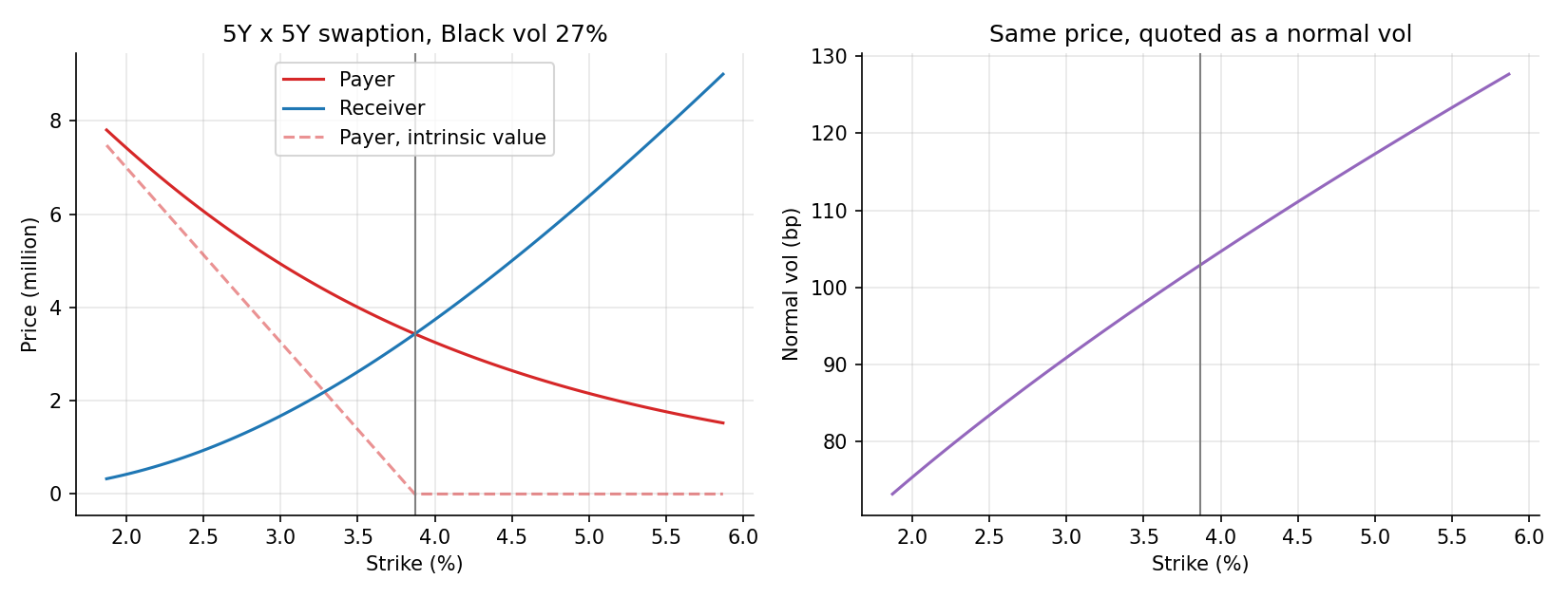
Payer and receiver swaption prices against strike, and the equivalent normal volatility — Left: Black prices against strike, with the payer’s intrinsic value as a dashed line. The gap above it is the time value. Right: the normal volatility that gives the same price as a constant 27% Black volatility.#

Reading the output:

The payer and receiver are equal at the money, because the forward swap is worth zero.
The parity gap is zero to rounding, as it should be.
The same 27% Black volatility is a different normal volatility at each strike (89, 103 and 116 basis points), because the two conventions measure the same price in different units. At the money it is close to \(0.27 \times 3.87\% = 104.5\) basis points.
The delta is the change in the price for a 1 basis point rise in the forward swap rate, and the vega is the change for a 1 point rise in the volatility. They are the risks that the desk hedges, and that valuation control sees in the sensitivity reports.

Greeks and conventions#

Delta: \(A \, N(d_1)\) per unit of rate for a payer, which is the hedge ratio against the forward swap rate.
Vega: \(A \, F \, n(d_1) \sqrt{T}\), which is largest at the money and for long expiries.
Quotation: swaption volatilities are quoted at the money, with offsets in basis points for other strikes. Most markets now quote normal volatilities.
Settlement: a physically settled swaption delivers a swap. A cash-settled one pays the value of the swap using a market formula, which changes the annuity used.
Premium and day counts: a mismatch in the accrual convention between the model and the market is a common source of small breaks.

A valuation control view#

For vanilla swaptions, IPV compares the desk’s volatility with independent consensus data by expiry, tenor and strike. Points to check:

Quote basis: the desk and the source must use the same convention (normal or lognormal, the same strike offset, the same forward). A difference in basis looks like a price break.
Parity and consistency: payer and receiver must be consistent, and the volatility cube must not have gaps or kinks between its points.
Observability: short-expiry, medium-tenor at-the-money points are liquid, so they are Level 2. Long expiry, long tenor and far-from-the-money strikes may be thin. Their observability decides the level in Fair-value hierarchy: Levels 1, 2 & 3.
Reserves: where there is no data, a model reserve or a prudent valuation adjustment covers the uncertainty. See Prudent Valuation.