SABR: Modelling the Volatility Smile#

Why a smile exists#

If rates followed the Black model, the implied volatility would be the same at all strikes. In practice:

Skew: volatility is higher for low strikes than for high strikes in many markets, because a fall in rates, and the move toward zero, behaves differently from a rise.
Curvature: volatility rises far from the money in both directions, because large moves are more likely than a lognormal model suggests.

A model that is used to price anything away from the money, or to price exotic options that depend on the smile, has to reproduce it.

The model#

SABR stands for “stochastic alpha, beta, rho”. The forward rate \(F\) and its volatility \(\alpha\) both move randomly:

\[dF = \alpha F^{\beta} \, dW_1\]

\[d\alpha = \nu \alpha \, dW_2, \qquad dW_1 \, dW_2 = \rho \, dt\]

There are four parameters, and each has a clear effect on the smile:

The SABR parameters#
Parameter	Meaning	Effect on the smile
\(\alpha\)	The initial level of volatility.	Moves the whole smile up or down. It is mostly set by the at-the-money volatility.
\(\beta\)	The “backbone”: how the volatility of the rate depends on its level. 1 is lognormal, 0 is normal.	Sets how the at-the-money volatility moves when the forward rate moves. It also adds some skew.
\(\rho\)	The correlation between the rate and its volatility.	Controls the skew. A negative value makes low strikes more expensive than high ones.
\(\nu\)	The volatility of volatility (“volvol”).	Controls the curvature. A larger value gives a stronger smile in both directions.

Choosing beta#

\(\beta\) and \(\rho\) both produce skew, so a calibration cannot tell them apart from a single smile. The usual practice is to fix \(\beta\) in advance and calibrate the other three. The common choices are:

0.5, a compromise between normal and lognormal behaviour, which was the traditional default
0, a normal backbone, which is natural where rates can be negative
a value chosen from the history of the at-the-money volatility against the rate level

Fixing \(\beta\) is a modelling decision that changes the prices, the Greeks and the parameters, so it must be recorded as part of the methodology.

Three features of the smile, three parameters#

A smile at one expiry can be described by three numbers. They are measured from the quoted volatilities, and each one is mostly controlled by one SABR parameter:

Smile features and the parameter that fits each#
Feature	How to measure it	Example, 5Y x 5Y	Parameter
Level	The at-the-money volatility.	26.8%	\(\alpha\)
Skew	The slope: the volatility at a low strike less the volatility at a high strike, for example -100 and +100 basis points.	30.4% less 25.4% = 5.0 points	\(\rho\)
Curvature	The convexity: the average of the two wing volatilities less the at-the-money volatility.	27.9% less 26.8% = 1.1 points	\(\nu\)

The figure shows each parameter moved on its own, with the other two fixed. \(\alpha\) shifts the whole curve up or down. \(\rho\) tilts it. \(\nu\) bends it, and a large value lifts both wings.

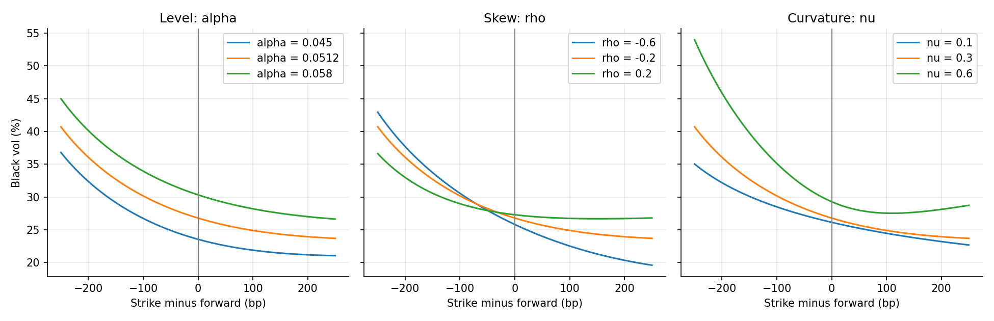
Three panels showing the SABR smile as alpha, rho and nu are changed one at a time — The effect of each SABR parameter on the smile, with \(\beta = 0.5\).#

Three features need three parameters, so a calibration to one smile has exactly enough freedom and no more. That is why \(\beta\) is fixed and not fitted. It also changes the skew, so a fit that tried to find \(\beta\) and \(\rho\) together would trade one against the other and give unstable, hard-to-interpret answers. With \(\beta\) fixed in advance, the three parameters \(\alpha\), \(\rho\) and \(\nu\) are each tied to a feature that can be read from the quotes. A good first check on any calibration is whether the fitted parameters reproduce those three numbers.

Calibration#

For each expiry and tenor, the model is fitted to the market volatilities at several strikes. The procedure:

Fix \(\beta\).
Take the market implied volatilities at a set of strikes, often the at-the-money quote and offsets such as -200, -100, -50, +50, +100 and +200 basis points.
Compute the model volatility at each strike using Hagan’s approximation (see Hagan’s Approximation: From SABR to a Black Volatility).
Adjust \(\alpha\), \(\rho\) and \(\nu\) to minimise the squared difference between model and market, with bounds such as \(-1 < \rho < 1\) and \(\alpha, \nu > 0\).

Many desks solve for \(\alpha\) so that the at-the-money volatility is matched exactly, and then fit \(\rho\) and \(\nu\) to the wings. The parameters are then interpolated across expiry and tenor to give a volatility cube.

Worked example#

The script fits SABR with \(\beta = 0.5\) to seven quoted volatilities for the 5Y x 5Y swaption, and then checks the fit and the implied probability density. The quotes are invented, with a skew and some noise so that the fit is not perfect. It uses the forward swap rate from Interest Rate Curve Build and the Black and normal volatility functions from Swaptions and the Black-76 Model.

"""SABR: Hagan's implied-vol approximation, calibration to a smile, and a no-arbitrage check."""
import numpy as np
from scipy.optimize import least_squares

from curve_example import bootstrap, forward_swap
from swaption_example import black_price, normal_vol_equivalent


def sabr_black_vol(forward, strike, expiry, alpha, beta, rho, nu, shift=0.0):
    """Hagan et al. (2002) lognormal implied vol. A positive `shift` handles low or negative rates."""
    f, k = forward + shift, np.asarray(strike, dtype=float) + shift
    log_fk = np.log(f / k)
    fk_mid = (f * k) ** ((1.0 - beta) / 2.0)
    z = nu / alpha * fk_mid * log_fk
    sqrt_term = np.sqrt(1.0 - 2.0 * rho * z + z**2)
    x_z = np.log((sqrt_term + z - rho) / (1.0 - rho))
    # z / x(z) tends to 1 at the money, where both are zero.
    z_over_x = np.where(np.abs(z) < 1e-7, 1.0, z / np.where(np.abs(z) < 1e-7, 1.0, x_z))
    denominator = fk_mid * (1.0 + (1.0 - beta) ** 2 / 24.0 * log_fk**2 + (1.0 - beta) ** 4 / 1920.0 * log_fk**4)
    correction = 1.0 + (
        (1.0 - beta) ** 2 / 24.0 * alpha**2 / fk_mid**2
        + rho * beta * nu * alpha / (4.0 * fk_mid)
        + (2.0 - 3.0 * rho**2) / 24.0 * nu**2
    ) * expiry
    return alpha / denominator * z_over_x * correction


def calibrate(forward, strikes, market_vols, expiry, beta, start=(0.05, -0.2, 0.3)):
    """Fit alpha, rho and nu to the smile, with beta fixed."""

    def residuals(p):
        return sabr_black_vol(forward, strikes, expiry, p[0], beta, p[1], p[2]) - market_vols

    fit = least_squares(residuals, start, bounds=([1e-4, -0.999, 1e-3], [1.0, 0.999, 3.0]))
    return fit.x, fit.fun


def call_density(forward, strikes, expiry, annuity, vol_function, step=1e-4):
    """Second derivative of the call price in strike. It is the risk-neutral density, so it must be >= 0."""
    price = lambda k: black_price(forward, k, vol_function(k), expiry, annuity, payer=True)
    return (price(strikes + step) - 2.0 * price(strikes) + price(strikes - step)) / step**2 / annuity


if __name__ == "__main__":
    curve = bootstrap()
    expiry, tenor, beta = 5.0, 5, 0.5
    forward, annuity = forward_swap(curve, expiry, tenor)

    offsets_bp = np.array([-200, -100, -50, 0, 50, 100, 200])
    strikes = forward + offsets_bp / 1e4
    market_vols = np.array([0.3560, 0.3040, 0.2830, 0.2680, 0.2600, 0.2540, 0.2480])  # quoted Black vols

    (alpha, rho, nu), errors = calibrate(forward, strikes, market_vols, expiry, beta)
    print(f"Forward {forward:.4%}, beta {beta}")
    print(f"alpha {alpha:.4f}, rho {rho:+.3f}, nu {nu:.3f}\n")

    fitted = sabr_black_vol(forward, strikes, expiry, alpha, beta, rho, nu)
    print(f"{'Offset':>7} {'Market':>8} {'SABR':>8} {'Error':>9} {'Normal vol':>11}")
    for bp, strike, market, model in zip(offsets_bp, strikes, market_vols, fitted):
        normal = normal_vol_equivalent(forward, strike, model, expiry, annuity) * 1e4
        print(f"{bp:+6d}bp {market:8.2%} {model:8.2%} {(model - market) * 100:+6.2f}pts {normal:9.1f}bp")
    print(f"\nRMS error: {np.sqrt(np.mean(errors**2)) * 100:.2f} vol points")

    # Density check across a wide strike range.
    grid = np.linspace(0.002, 0.10, 99)
    vol_function = lambda k: sabr_black_vol(forward, k, expiry, alpha, beta, rho, nu)
    density = call_density(forward, grid, expiry, annuity, vol_function)
    print(f"Lowest density on 0.2% to 10% strikes: {density.min():.3f}")

    # A longer expiry with the same parameters shows where the approximation breaks down.
    for long_expiry in (5.0, 20.0, 30.0):
        vol_function = lambda k, e=long_expiry: sabr_black_vol(forward, k, e, alpha, beta, rho, nu)
        density = call_density(forward, grid, long_expiry, annuity, vol_function)
        print(f"Expiry {long_expiry:4.0f}Y: lowest density {density.min():.3f}")

Running it gives:

Forward 3.8700%, beta 0.5
alpha 0.0512, rho -0.112, nu 0.307

 Offset   Market     SABR     Error  Normal vol
  -200bp   35.60%   35.71%  +0.11pts      95.7bp
  -100bp   30.40%   30.08%  -0.32pts      98.8bp
   -50bp   28.30%   28.30%  +0.00pts     100.6bp
    +0bp   26.80%   27.00%  +0.20pts     102.9bp
   +50bp   26.00%   26.07%  +0.07pts     105.8bp
  +100bp   25.40%   25.42%  +0.02pts     109.1bp
  +200bp   24.80%   24.71%  -0.09pts     117.2bp

RMS error: 0.15 vol points
Lowest density on 0.2% to 10% strikes: 0.887
Expiry    5Y: lowest density 0.887
Expiry   20Y: lowest density -71.446
Expiry   30Y: lowest density -66.633

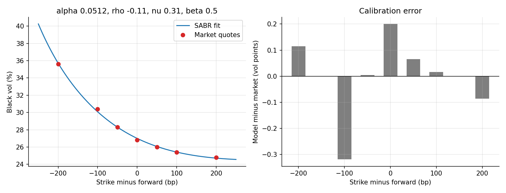
The fitted SABR smile against the seven market quotes, and the error at each strike — The calibrated smile with the quotes, and the error at each strike.#

Reading the output:

The fitted parameters are \(\alpha = 0.0512\), \(\rho = -0.112\) and \(\nu = 0.307\). The negative \(\rho\) gives the skew, and \(\nu\) gives the curvature.
The fit is within about a third of a volatility point at every strike. It is not exact, because three parameters are fitted to seven quotes. A large error at one strike is a prompt to check that quote.
The model at-the-money volatility is 27.0%, and that is the number used in Swaptions and the Black-76 Model.
The normal volatility column rises with the strike. The market quotes in the two conventions give different pictures of the same smile.
The last three lines are explained in Hagan’s Approximation: From SABR to a Black Volatility: the density from the fit is positive for 5 years, but the same parameters at long expiries give negative densities at low strikes.

Negative rates and shifted SABR#

The formula needs \(\ln(F/K)\) and \((FK)^{(1-\beta)/2}\), so it breaks when the forward rate or the strike is zero or negative. Euro, Swiss franc and yen rates were negative for years after 2014, and a rate close to zero is a problem even without a sign change. The standard fix is a shift. The model is applied to \(F + s\) instead of \(F\), for a fixed shift \(s\):

\[d(F + s) = \alpha (F + s)^{\beta} \, dW_1\]

Everything else is unchanged. The volatility formula in Hagan’s Approximation: From SABR to a Black Volatility is evaluated at \(F + s\) and \(K + s\), which are positive as long as \(s\) is larger than the most negative strike. The result is a shifted Black volatility, which goes into the Black formula with the shifted forward and strike. Because markets with negative rates quote normal volatilities, a calibration converts each quote to a shifted Black volatility first, and converts the model result back to compare with the market.

The shift is a modelling choice that is fixed in advance, like \(\beta\). The script below calibrates a shifted SABR, with \(\beta = 0.5\) and a shift of 3%, to a 5Y swaption on a forward swap rate of -0.25%. The quotes are invented normal volatilities in basis points. It also refits with other shifts.

"""Shifted SABR for negative rates: calibrate to normal-volatility quotes."""
import numpy as np
from scipy.optimize import brentq, least_squares

from sabr_example import sabr_black_vol
from swaption_example import bachelier_price, black_price


def shifted_black_vol(forward, strike, normal_vol, expiry, shift):
    """Shifted-lognormal vol that gives the same price as a normal vol quote."""
    target = bachelier_price(forward, strike, normal_vol, expiry, 1.0)
    return brentq(lambda v: black_price(forward + shift, strike + shift, v, expiry, 1.0) - target, 1e-4, 5.0)


def normal_vol_from_shifted(forward, strike, black_vol, expiry, shift):
    """The reverse: the normal vol that matches a shifted-lognormal vol."""
    target = black_price(forward + shift, strike + shift, black_vol, expiry, 1.0)
    return brentq(lambda v: bachelier_price(forward, strike, v, expiry, 1.0) - target, 1e-6, 0.05)


def calibrate_shifted(forward, strikes, normal_vols, expiry, beta, shift):
    """Fit alpha, rho and nu to normal-vol quotes, through the shifted Black vols."""
    market = np.array([shifted_black_vol(forward, k, v, expiry, shift) for k, v in zip(strikes, normal_vols)])

    def residuals(p):
        return sabr_black_vol(forward, strikes, expiry, p[0], beta, p[1], p[2], shift) - market

    start = (market[len(market) // 2] * (forward + shift) ** (1 - beta), -0.2, 0.3)
    fit = least_squares(residuals, start, bounds=([1e-4, -0.999, 1e-3], [1.0, 0.999, 3.0]))
    return fit.x


if __name__ == "__main__":
    forward, expiry, beta = -0.0025, 5.0, 0.5   # a forward swap rate below zero
    offsets_bp = np.array([-150, -100, -50, 0, 50, 100, 150])
    strikes = forward + offsets_bp / 1e4
    normal_vols = np.array([62.0, 58.5, 56.0, 55.0, 55.5, 57.5, 60.5]) / 1e4  # quoted normal vols

    with np.errstate(all="ignore"):
        unshifted = sabr_black_vol(forward, strikes, expiry, 0.03, beta, -0.2, 0.3)
    print(f"Forward {forward:.2%}. Unshifted SABR vols: {np.round(unshifted, 3)}\n")

    shift = 0.03
    alpha, rho, nu = calibrate_shifted(forward, strikes, normal_vols, expiry, beta, shift)
    print(f"Shift {shift:.0%}: alpha {alpha:.4f}, rho {rho:+.3f}, nu {nu:.3f}\n")
    print(f"{'Strike':>8} {'Market':>9} {'SABR':>9} {'Error':>8}")
    for strike, market in zip(strikes, normal_vols):
        vol = sabr_black_vol(forward, strike, expiry, alpha, beta, rho, nu, shift)
        model = normal_vol_from_shifted(forward, strike, float(vol), expiry, shift)
        print(f"{strike:8.2%} {market * 1e4:7.1f}bp {model * 1e4:7.1f}bp {(model - market) * 1e4:+6.2f}bp")

    # The shift is a free choice. It barely moves the quoted strikes but changes the wings, and a
    # strike at or below -shift cannot be priced at all.
    far_strike = -0.0200
    print(f"\n{'Shift':>6} {'alpha':>7} {'rho':>7} {'nu':>6} {'ATM':>8} {'K = -2.00%':>11}")
    for s in (0.02, 0.03, 0.05, 0.10):
        a, r, n = calibrate_shifted(forward, strikes, normal_vols, expiry, beta, s)
        atm = normal_vol_from_shifted(forward, forward, float(sabr_black_vol(forward, forward, expiry, a, beta, r, n, s)), expiry, s)
        if far_strike + s > 0:
            far_vol = float(sabr_black_vol(forward, far_strike, expiry, a, beta, r, n, s))
            far = f"{normal_vol_from_shifted(forward, far_strike, far_vol, expiry, s) * 1e4:9.1f}bp"
        else:
            far = "       n/a"
        print(f"{s:6.0%} {a:7.4f} {r:+7.3f} {n:6.3f} {atm * 1e4:6.1f}bp {far:>11}")

Running it gives:

Forward -0.25%. Unshifted SABR vols: [0.429 0.439 0.469 0.619   nan   nan   nan]

Shift 3%: alpha 0.0319, rho -0.343, nu 0.409

  Strike    Market      SABR    Error
  -1.75%    62.0bp    61.5bp  -0.48bp
  -1.25%    58.5bp    59.1bp  +0.63bp
  -0.75%    56.0bp    56.5bp  +0.53bp
  -0.25%    55.0bp    54.7bp  -0.26bp
   0.25%    55.5bp    54.8bp  -0.68bp
   0.75%    57.5bp    57.2bp  -0.33bp
   1.25%    60.5bp    61.2bp  +0.74bp

 Shift   alpha     rho     nu      ATM  K = -2.00%
    2%  0.0360  -0.467   0.757   51.6bp         n/a
    3%  0.0319  -0.343   0.409   54.7bp      62.3bp
    5%  0.0243  -0.225   0.346   54.9bp      63.4bp
   10%  0.0169  -0.131   0.326   54.9bp      63.7bp

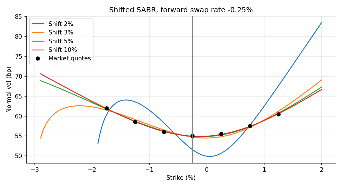
Shifted SABR normal volatility smiles for four shifts, against the market quotes — Shifted SABR fitted to the same quotes with four different shifts.#

Reading the output:

Without a shift the formula fails. The unshifted volatilities are NaN where the strike and the forward have opposite signs. Where both are negative the formula returns numbers, but they have no meaning, because the formula treats the negative rate as if it were positive.
With a 3% shift the fit is good. The errors are below 0.8 basis points of normal volatility at every strike. The parameters are different from the positive-rate example, as the shift changes the meaning of \(\alpha\).
A shift that is too small fails. With 2%, the shifted strike at -1.75% is only 0.25%, which is close to the singularity. The fit is poor, with an at-the-money volatility of 51.6 basis points against a quote of 55, and a strike of -2.00% cannot be priced at all, as it equals \(-s\).
The quoted strikes hardly depend on the shift once it is large enough, as shifts of 3%, 5% and 10% give the same at-the-money volatility to within a fraction of a basis point.
The wings do depend on it. Far from the money, at -2.00%, the volatilities are 62.3, 63.4 and 63.7 basis points for 3%, 5% and 10%. Near the lower limit of the range, the 3% curve in the figure falls away sharply, which is a sign that the strike is too close to \(-s\). A larger shift is stable over a wider range of strikes, but it makes the model behave more like a normal model, and it changes the implied skew.

Choosing the shift#

It must be larger than the most negative strike or forward that the model has to price, with a margin. Rates can fall further, so a limit that is breached is a model failure and not a rounding error.
It is a convention in many markets, with a standard amount for each currency, so that all desks calibrate and quote on the same basis.
The calibration and the pricing must use the same shift. A mismatch is a common bug.
An alternative is \(\beta = 0\), the normal SABR, which allows negative rates without a shift.

Using the fitted smile#

Once calibrated, SABR gives a volatility for any strike, which is put in the Black formula to get a price. That serves several purposes:

Pricing and marking swaptions away from the quoted strikes, including interpolating the strike dimension of the cube.
Risk: the sensitivity to the parameters, and to the forward rate with the smile moving with it. Vega is split into the sensitivity to \(\alpha\), \(\rho\) and \(\nu\).
Replication of exotic payoffs, such as constant maturity swap (CMS) products and caps and floors, with the static replication of a payoff by a strip of swaptions priced from the smile.

Limits of SABR#

It is a model for one forward rate at one expiry. It does not give a dynamic description of the whole curve, so it does not by itself price a Bermudan or an option on several rates. See Bermudan Swaptions and Mean Reversion.
The parameters are not stable, and \(\rho\) and \(\nu\) can jump when the market moves.
Very low rates, and negative rates, need a normal backbone or a shift.
The popular approximation can give negative densities for long expiries and low strikes. See Hagan’s Approximation: From SABR to a Black Volatility.

A valuation control view#

SABR is a model, so it comes under model risk governance. See Governance: Model Risk, Accountability and Data. For IPV and model control:

Fit quality: the errors at each quote, by expiry and tenor, are reviewed against a tolerance. A systematic misfit at the wings means the model is not capturing the smile.
Parameter stability: \(\alpha\), \(\rho\) and \(\nu\) are plotted over time and across the cube. Jumps point to bad quotes or an unstable fit.
Choice of beta: it is documented, and its effect on the price is tested. A different \(\beta\) with a refit should give similar prices at the quoted strikes and different prices away from them. The difference is a measure of model uncertainty.
Extrapolation: prices far from the quoted strikes come from the model, not the market. This is a model reserve or a prudent valuation adjustment, and an input to the level. See Prudent Valuation and Fair-value hierarchy: Levels 1, 2 & 3.
Arbitrage checks: the implied density must not be negative, and the call price must be convex in strike.