Interest Rate Curve Build#

What the curve is#

The discount factor \(D(t)\) is the value today of 1 paid at time \(t\). The other quantities come from it:

\[z(t) = -\frac{\ln D(t)}{t}, \qquad f(t_1, t_2) = \frac{\ln D(t_1) - \ln D(t_2)}{t_2 - t_1}\]

\(z(t)\) is the continuously compounded zero rate to \(t\), and \(f(t_1,t_2)\) is the forward rate between two dates. Both are different ways to express the same curve.

Instruments#

The curve is built from the most liquid instruments at each maturity.

Typical inputs#
Instrument	Maturity range	Use
Overnight rate and deposits	Up to about 3 months	Sets the very short end.
Futures or FRAs	Up to about 2 to 3 years	Gives forward rates in the short end. Futures need a convexity adjustment.
Overnight index swaps (OIS)	1 week to 50 years	A fixed rate against compounded overnight rates, such as SOFR or SONIA. This is the core of a modern curve.
Basis swaps	1 year and longer	Link the overnight curve to a term curve, or one currency to another.

Since the move from LIBOR to overnight rates, the main USD curve is SOFR and the main GBP curve is SONIA. For these swaps the floating leg is the overnight rate itself, so its value is simple, as shown below.

Bootstrapping#

Bootstrapping solves for the discount factors one pillar at a time, from the shortest to the longest, so that each input reprices to par. For an overnight index swap with annual fixed payments of rate \(s\) and maturity \(T_n\):

\[s \sum_{i=1}^{n} \tau_i D(T_i) = 1 - D(T_n)\]

The left side is the fixed leg. The right side is the floating leg, which is worth 1 less the discount factor at maturity because compounding an overnight rate and discounting at the same curve cancels. For a given pillar, all of the discount factors before it are already known, so there is one unknown, \(D(T_n)\). The equation is solved for it, for example by a root finder.

Between pillars there are dates with no quote, such as the annual payment dates between the 7 and 10 year swaps. Their discount factors come from the interpolation rule, which is part of the curve.

Interpolation#

Common interpolation choices#
Method	Property	Weakness
Linear in the discount factor	Simple.	Gives forward rates with large jumps.
Log-linear in the discount factor	Flat forward rates between pillars. Never gives negative forwards when the inputs are sensible.	Forward curve is a staircase, so it is not smooth and hedge risk jumps at the pillars.
Linear in the zero rate	Smooth zero curve.	Forward rates can oscillate and go negative.
Cubic splines, monotone convex	Smooth, with sensible forward rates. Monotone convex is built to stay positive and local.	More complex. A poor spline can oscillate.

The choice changes the forward rates, and so changes the price of anything that depends on them, such as a forward-starting swap or a swaption. It must be documented and be the same across the firm.

Worked example#

The script bootstraps a curve from nine par swap rates, with annual fixed payments and log-linear discount factors, and reprices the inputs. The single-curve set-up is exact here because the floating leg is an overnight rate. The rates are invented but realistic.

"""Bootstrap a discount curve from par swap rates, then reprice the inputs as a check."""
import numpy as np
from scipy.optimize import brentq

PILLARS = [1, 2, 3, 5, 7, 10, 15, 20, 30]  # years
PAR_RATES = [0.0400, 0.0380, 0.0370, 0.0365, 0.0368, 0.0375, 0.0385, 0.0380, 0.0365]


class Curve:
    """Discount factors, interpolated log-linearly (flat forward rates between pillars)."""

    def __init__(self, times, dfs):
        self.t = np.concatenate([[0.0], times])
        self.d = np.concatenate([[1.0], dfs])

    def df(self, t):
        return np.exp(np.interp(t, self.t, np.log(self.d)))


def bootstrap(pillars=PILLARS, par_rates=PAR_RATES):
    """Solve for one discount factor per pillar, so that each par swap reprices to zero."""
    times, dfs = [], []
    for maturity, rate in zip(pillars, par_rates):

        def error(df_maturity):
            curve = Curve(times + [maturity], dfs + [df_maturity])
            annual_dates = np.arange(1, maturity + 1)
            # Annual fixed leg against an overnight floating leg worth 1 - DF(maturity).
            return rate * curve.df(annual_dates).sum() - (1.0 - df_maturity)

        dfs.append(brentq(error, 1e-6, 1.0))
        times.append(maturity)
    return Curve(times, dfs)


def forward_swap(curve, expiry, tenor):
    """Forward par swap rate and annuity for an annual fixed leg starting at `expiry`."""
    pay_dates = expiry + np.arange(1, tenor + 1)
    annuity = curve.df(pay_dates).sum()
    return (curve.df(expiry) - curve.df(pay_dates[-1])) / annuity, annuity


if __name__ == "__main__":
    curve = bootstrap()

    print(f"{'Pillar':>6} {'Par rate':>9} {'DF':>9} {'Zero':>8} {'Fwd':>8}")
    previous_t, previous_df = 0.0, 1.0
    for t, rate in zip(PILLARS, PAR_RATES):
        df = curve.df(t)
        zero = -np.log(df) / t
        forward = np.log(previous_df / df) / (t - previous_t)
        print(f"{t:>5}Y {rate:9.4%} {df:9.6f} {zero:8.4%} {forward:8.4%}")
        previous_t, previous_df = t, df

    # Reprice every input swap with the finished curve.
    errors = []
    for t, rate in zip(PILLARS, PAR_RATES):
        repriced, _ = forward_swap(curve, 0, t)
        errors.append(abs(repriced - rate))
    print(f"\nLargest repricing error: {max(errors):.2e}")

    forward, annuity = forward_swap(curve, 5, 5)
    print(f"5Y x 5Y forward swap rate: {forward:.4%}, annuity: {annuity:.4f}")

Running it gives:

Pillar  Par rate        DF     Zero      Fwd
    1Y   4.0000%  0.961538  3.9221%  3.9221%
    2Y   3.8000%  0.928190  3.7259%  3.5298%
    3Y   3.7000%  0.896895  3.6272%  3.4298%
    5Y   3.6500%  0.836160  3.5787%  3.5060%
    7Y   3.6800%  0.776581  3.6122%  3.6960%
   10Y   3.7500%  0.691434  3.6899%  3.8711%
   15Y   3.8500%  0.565090  3.8051%  4.0357%
   20Y   3.8000%  0.473998  3.7328%  3.5156%
   30Y   3.6500%  0.348178  3.5168%  3.0849%

Largest repricing error: 3.10e-14
5Y x 5Y forward swap rate: 3.8700%, annuity: 3.7397

The forward column is the flat forward between each pillar and the one before. It moves around from one segment to the next, which shows the staircase shape of log-linear interpolation. The last line is the 5-year forward swap rate starting in 5 years. It is used in Swaptions and the Black-76 Model, and the other pages in this series.

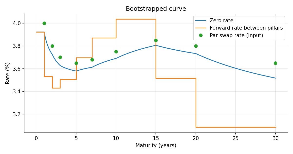
Zero rate curve, step-shaped forward rates and the par swap rate inputs — The bootstrapped zero curve and the flat forwards between pillars. The par rates are the inputs. The forwards are above the zero rate when the curve is rising and below it when it is falling.#

Beyond the basic curve#

This section lists the main extensions. Curve Build, Part 2: Jacobians, Global Solvers and Multi-Curve covers multi-curve, global solvers, the Jacobian and interpolation in detail. * Multi-curve: before 2008 one curve served both for discounting and for projecting floating rates. Today the discount curve follows the collateral rate, which is an overnight rate, and the projection curves for each tenor of an index are separate. Overnight-index products such as SOFR swaps need only one. * Collateral and currency: the discount curve depends on the currency and the terms of the collateral agreement, which links curve choice to ColVA: Collateral Valuation Adjustment. * Turn-of-year and holidays: the short end has jumps at the end of a quarter or a year. Business-day and day-count conventions matter at the level of basis points. * Risk: the sensitivity to each input (a bucketed DV01 or a Jacobian) comes from the bootstrap, so it is easy to report risk by pillar. * Extrapolation: beyond the last liquid pillar, which is often 30 or 50 years, the curve is an assumption and needs its own control.

A valuation control view#

The curve underlies everything else, so the controls are about inputs and methodology:

Inputs: each instrument’s quote is checked against an independent source at the same snapshot time, with a tolerance by tenor.
Repricing: the curve must reprice its inputs to a small tolerance, as in the check above. A repricing break means a bug or a stale input.
Smoothness: the forward curve is inspected for jumps, negative forwards or kinks that are not in the market.
Methodology: the interpolation, the day counts and the choice of curves are documented and approved. See Governance: Model Risk, Accountability and Data.
Link to fair value: quotes that are illiquid, such as 30 year and longer pillars, are an input to the level judgement in Fair-value hierarchy: Levels 1, 2 & 3.