Bermudan Swaptions and Mean Reversion#

The product#

A “10NC2” Bermudan payer swaption is a swap that runs for 10 years, with the right to enter it from year 2 onwards. At each annual date between years 2 and 9 the holder can exercise, and the swap that is entered then runs to the common end date, year 10. These underlying swaps all end on the same date, so they are called co-terminal.

The value has two parts:

the European swaptions on the co-terminal swaps, each exercisable on one date
the switch option, which is the extra value of being able to choose the best date, instead of fixing one in advance

Black-76 and SABR cannot price this. They value each European separately and have no view of how the rates at different dates move together. A Bermudan needs a model of the whole curve over time, so that the decision to exercise at one date can be compared with the value of waiting.

Why a model is needed#

At each exercise date, the holder compares the value of exercising now with the value of keeping the option. The value of keeping it depends on what the rates are likely to do next, which means on the correlation between the rates on different dates. If the rate at year 5 tells you a lot about the rate at year 6, there is little value in waiting, and if it tells you little, waiting is worth more. A one-factor short-rate model describes this through its mean reversion.

The Hull-White model#

The Hull-White one-factor model describes the short rate \(r(t)\):

\[dr = \left[ \theta(t) - a \, r \right] dt + \sigma \, dW\]

\(a\) is the mean reversion speed. When the rate is above its long-run level, the drift pulls it down at rate \(a\).
\(\sigma\) is the volatility of the short rate.
\(\theta(t)\) is a function of time, chosen so that the model reprices today’s discount curve exactly. This is what makes the model consistent with the curve from Interest Rate Curve Build.

Bond prices are available in closed form, so the model is fast, and European swaptions have a closed-form price too. This is Jamshidian’s decomposition, in which a swaption is a sum of options on zero-coupon bonds. That allows a quick calibration to European swaption prices.

What mean reversion does#

Mean reversion controls how rates at different times move together:

With no mean reversion (\(a = 0\)), the short rate is a random walk and a shock has a permanent effect. Rates at different dates are highly correlated, and the spread of possible rates keeps growing with the horizon.
With high mean reversion, a shock fades. The effect is that long-term rates are much less volatile than short-term rates, and rates at different times are less correlated.

\(a\) and \(\sigma\) trade off against each other. A larger \(a\) needs a larger \(\sigma\) to give the same price for a given European swaption, because the shocks decay faster. A single European price therefore cannot pin down both.

Calibration#

The usual approach is to calibrate to the co-terminal European swaptions, which are the options that make up the Bermudan, at the Bermudan’s strike. They are the closest hedges.

If \(a\) is fixed, \(\sigma\) is chosen, as a function of time if needed, so that the model prices each European to the market.
\(a\) is the main modelling choice. It is set from the market’s view of correlation, for example by calibrating to a second set of swaptions with a longer tenor, or by a policy value from the desk. It decides how the switch option is valued.

Because \(a\) is not pinned down by the co-terminal Europeans, two models that match every European price exactly can give different Bermudan prices. This is a known source of model risk and the reason for a reserve.

Pricing on a tree#

A tree gives the price directly. The short rate is represented on a recombining trinomial tree, which is fitted to the discount curve. At each exercise date the price of the option is the larger of the value of exercising, which is the value of the underlying swap at that node, and the value of continuing, which is the discounted expectation of the next step. Working backwards from the end gives the price today.

The steps are:

Build the tree for the process, with monthly steps, so that annual exercise dates fall on tree dates.
Fit the drift at each step so that the tree reproduces the discount factor for that date. This is done by forward induction with the state prices of each node.
Value the cash flows of the underlying swap at each node by backward induction.
Work backward and, at each exercise date, take the maximum of exercising and continuing.

Other methods exist. A finite-difference solution of the same model gives similar results. Monte Carlo is used with the regression method of Longstaff and Schwartz for multi-factor models, where a tree is too slow.

Worked example#

The script prices a 10NC2 Bermudan payer swaption, with annual exercise from year 2 to year 9 and a strike at the 5Y x 5Y forward swap rate of 3.87%, for 100 million of notional. It uses the curve from Interest Rate Curve Build.

First it checks the tree against the closed form for a European swaption. Then, for four values of mean reversion, it sets \(\sigma\) so that the model matches the Black price of the 5Y x 5Y swaption from Swaptions and the Black-76 Model, and prices the Bermudan.

"""Bermudan swaption on a Hull-White trinomial tree, and the effect of mean reversion."""
import numpy as np
from scipy.optimize import brentq
from scipy.stats import norm

from curve_example import bootstrap, forward_swap
from swaption_example import black_price

DT = 1.0 / 12.0  # monthly steps, so every annual exercise date falls on a tree date


def build_tree(curve, a, sigma, n_steps):
    """Hull-White tree for x, where r = alpha(t) + x. Alpha is fitted so the tree reprices the curve."""
    v = sigma**2 * (1.0 - np.exp(-2.0 * a * DT)) / (2.0 * a)
    dx = np.sqrt(3.0 * v)
    m = np.exp(-a * DT) - 1.0
    j_max = min(int(np.ceil(0.184 / (a * DT))), n_steps)
    j = np.arange(-j_max, j_max + 1)
    k = np.arange(len(j))

    # Standard branching: up, middle, down. The outermost nodes branch inward once the tree is truncated.
    pu = 1 / 6 + (j**2 * m**2 + j * m) / 2
    pm = 2 / 3 - j**2 * m**2
    pd = 1 / 6 + (j**2 * m**2 - j * m) / 2
    tu, tm, td = k + 1, k, k - 1
    if j_max == int(np.ceil(0.184 / (a * DT))):
        top, bottom = j == j_max, j == -j_max
        pu[top], pm[top], pd[top] = [
            7 / 6 + (j[top] ** 2 * m**2 + 3 * j[top] * m) / 2,
            -1 / 3 - j[top] ** 2 * m**2 - 2 * j[top] * m,
            1 / 6 + (j[top] ** 2 * m**2 + j[top] * m) / 2,
        ]
        tu[top], tm[top], td[top] = k[top], k[top] - 1, k[top] - 2
        pu[bottom], pm[bottom], pd[bottom] = [
            1 / 6 + (j[bottom] ** 2 * m**2 - j[bottom] * m) / 2,
            -1 / 3 - j[bottom] ** 2 * m**2 + 2 * j[bottom] * m,
            7 / 6 + (j[bottom] ** 2 * m**2 - 3 * j[bottom] * m) / 2,
        ]
        tu[bottom], tm[bottom], td[bottom] = k[bottom] + 2, k[bottom] + 1, k[bottom]
    last = len(j) - 1
    tu, tm, td = (np.clip(x, 0, last) for x in (tu, tm, td))

    # Forward induction: state prices Q, and alpha chosen at each step to match the discount factor.
    q = np.zeros(len(j))
    q[j_max] = 1.0
    alphas = np.zeros(n_steps)
    for i in range(n_steps):
        alphas[i] = (np.log(np.sum(q * np.exp(-j * dx * DT))) - np.log(curve.df((i + 1) * DT))) / DT
        flow = q * np.exp(-(alphas[i] + j * dx) * DT)
        q = np.zeros(len(j))
        np.add.at(q, tu, flow * pu)
        np.add.at(q, tm, flow * pm)
        np.add.at(q, td, flow * pd)
    return dict(j=j, dx=dx, alphas=alphas, pu=pu, pm=pm, pd=pd, tu=tu, tm=tm, td=td)


def price_payer(tree, strike, exercise_steps, n_steps, steps_per_year=12):
    """Bermudan payer swaption price per unit notional, by backward induction on the tree."""
    j, dx = tree["j"], tree["dx"]
    swap_end = n_steps
    cashflow = np.zeros(n_steps + 1)
    cashflow[steps_per_year::steps_per_year] = -strike  # annual fixed coupons paid
    cashflow[swap_end] -= 1.0                           # the notional that closes the floating leg

    u = np.zeros(len(j))      # value of the remaining swap cash flows
    option = np.zeros(len(j))
    for i in range(n_steps - 1, -1, -1):
        disc = np.exp(-(tree["alphas"][i] + j * dx) * DT)
        expect = lambda v: tree["pu"] * v[tree["tu"]] + tree["pm"] * v[tree["tm"]] + tree["pd"] * v[tree["td"]]
        u = disc * expect(u + cashflow[i + 1])
        option = disc * expect(option)
        if i in exercise_steps:
            option = np.maximum(option, 1.0 + u)  # exercise into the payer swap
    return option[tree["j"] == 0][0]


def jamshidian(curve, a, sigma, strike, expiry, swap_end):
    """Closed-form European Hull-White payer swaption, as a put on a coupon bond."""
    pay = np.arange(expiry + 1, swap_end + 1)
    coupons = np.full(len(pay), strike)
    coupons[-1] += 1.0
    b = lambda t, T: (1.0 - np.exp(-a * (T - t))) / a
    eps = 1e-4
    f0 = -(np.log(curve.df(expiry + eps)) - np.log(curve.df(expiry - eps))) / (2 * eps)

    def bond(T, r):
        log_a = (np.log(curve.df(T) / curve.df(expiry)) + b(expiry, T) * f0
                 - sigma**2 / (4 * a) * (1 - np.exp(-2 * a * expiry)) * b(expiry, T) ** 2)
        return np.exp(log_a - b(expiry, T) * r)

    r_star = brentq(lambda r: np.sum(coupons * bond(pay, r)) - 1.0, -0.5, 0.5)
    sigma_p = sigma * np.sqrt((1 - np.exp(-2 * a * expiry)) / (2 * a)) * b(expiry, pay)
    x = bond(pay, r_star)
    h = np.log(curve.df(pay) / (curve.df(expiry) * x)) / sigma_p + sigma_p / 2
    puts = x * curve.df(expiry) * norm.cdf(-h + sigma_p) - curve.df(pay) * norm.cdf(-h)
    return np.sum(coupons * puts)


if __name__ == "__main__":
    curve = bootstrap()
    n_steps, notional = 120, 100e6                 # 10 years, monthly
    forward, annuity = forward_swap(curve, 5, 5)
    strike = forward                              # at the money for the 5Y x 5Y co-terminal swaption
    target = black_price(forward, strike, 0.27, 5.0, annuity)

    # Check the tree against the closed form for a European 5Y x 5Y payer swaption.
    sigma_check, a_check = 0.0100, 0.05
    tree = build_tree(curve, a_check, sigma_check, n_steps)
    europe_tree = price_payer(tree, strike, {60}, n_steps)
    europe_closed = jamshidian(curve, a_check, sigma_check, strike, 5, 10)
    print(f"European check (a={a_check}, sigma={sigma_check:.2%}): tree {notional * europe_tree:,.0f}, "
          f"closed form {notional * europe_closed:,.0f}\n")

    # For each mean reversion, set sigma so the model matches the 5Y x 5Y swaption, then price the Bermudan.
    print(f"Black price of the 5Y x 5Y swaption to match: {notional * target:,.0f}\n")
    print(f"{'Mean rev':>9} {'Sigma':>8} {'Euro 5Yx5Y':>12} {'Bermudan':>12} {'Switch value':>13}")
    bermudan_steps = {12 * year for year in range(2, 10)}  # exercise annually from year 2 to year 9
    for a in (0.01, 0.03, 0.05, 0.10):
        def error(sigma):
            return price_payer(build_tree(curve, a, sigma, n_steps), strike, {60}, n_steps) - target

        sigma = brentq(error, 1e-4, 0.05)
        tree = build_tree(curve, a, sigma, n_steps)
        europe = price_payer(tree, strike, {60}, n_steps)
        bermudan = price_payer(tree, strike, bermudan_steps, n_steps)
        print(f"{a:9.2f} {sigma:8.3%} {notional * europe:12,.0f} {notional * bermudan:12,.0f} "
              f"{notional * (bermudan - europe):13,.0f}")

Running it gives:

European check (a=0.05, sigma=1.00%): tree 2,737,582, closed form 2,726,321

Black price of the 5Y x 5Y swaption to match: 3,433,592

 Mean rev    Sigma   Euro 5Yx5Y     Bermudan  Switch value
     0.01   1.040%    3,433,592    4,949,469     1,515,877
     0.03   1.143%    3,433,592    5,049,631     1,616,039
     0.05   1.254%    3,433,592    5,151,383     1,717,792
     0.10   1.563%    3,433,592    5,414,469     1,980,877

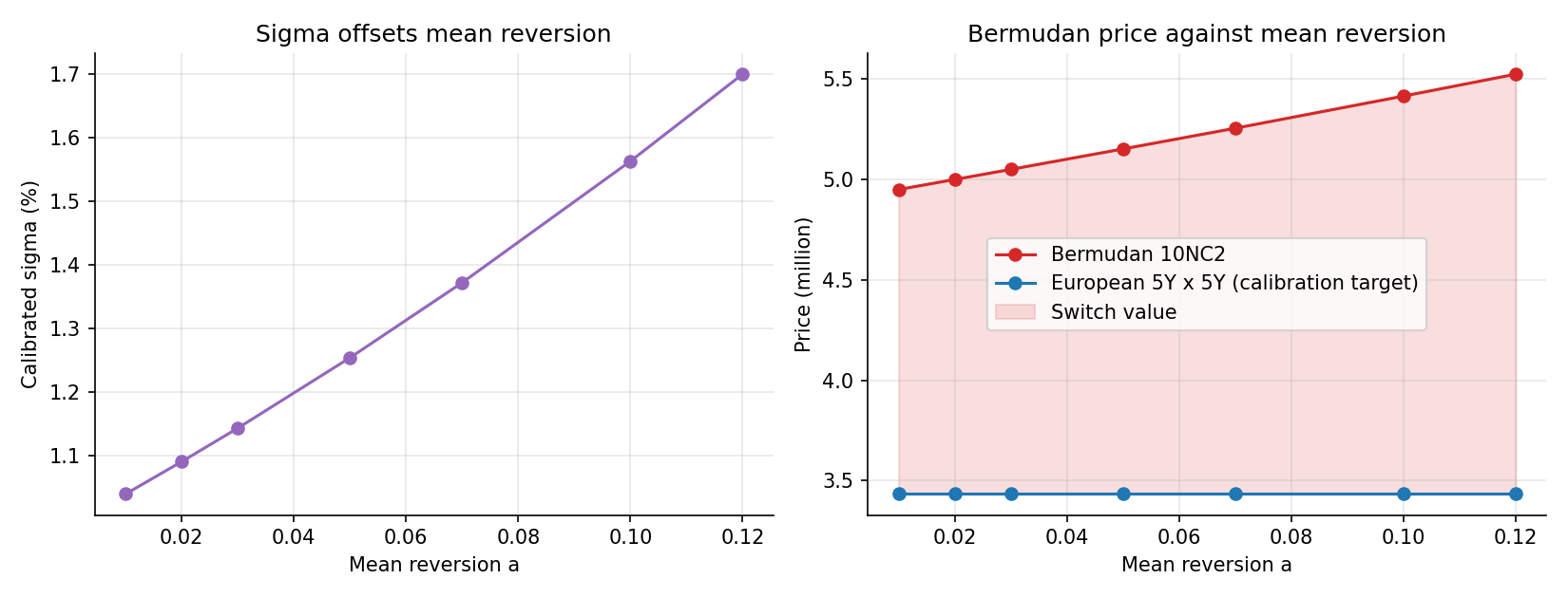
Calibrated sigma and Bermudan price against mean reversion, with the European swaption price as the floor — Calibrated sigma, and the Bermudan price against mean reversion. The shaded gap between the two lines on the right is the switch value.#

Reading the output:

The tree check. The tree and the closed form differ by about 0.4%. The difference is the discretisation of the tree, and it shrinks as the steps are made smaller. In a separate test that is not in the script, halving the step size once and then twice cut the gap to about 0.2% and then 0.08%.
The Bermudan is worth more than the European. At every mean reversion, the Bermudan is above the 3.43 million of the European that was used for calibration, and the excess is the switch value.
Sigma rises with mean reversion. To match the same European price, \(\sigma\) goes from 1.04% to 1.56% as \(a\) rises from 0.01 to 0.10. The two parameters offset each other.
The Bermudan price rises with mean reversion. With the same calibration, the price goes from 4.95 million to 5.41 million, which is 9% higher. A higher \(a\) gives less correlation between the rates at different dates, so the exercise decision is worth more.

So two models that fit the same European swaption can differ by 0.47 million on the Bermudan, which is the measure of model uncertainty to be understood. In practice the model is calibrated to all of the co-terminal Europeans, which narrows the difference, but does not remove it, because the correlation between the dates is still a choice.

Risk and hedging#

Delta and vega: the Bermudan has sensitivity to the curve and to the volatility of each co-terminal swaption, so the hedge is a portfolio of European swaptions.
Mean reversion risk: the price depends on \(a\), which is not hedgeable with vanilla instruments. This is a model risk and is usually managed as a reserve.
Exercise boundary: a rate level at each date above or below which the holder exercises. It shows the economic logic and is a useful check on the model output.

A valuation control view#

A Bermudan swaption is typically a Level 2 or Level 3 position. The inputs, the co-terminal European volatilities, may be observable. The value depends on a model parameter, the mean reversion, that is not, so the controls are:

Independent model: a separate implementation, for example a different numerical method, is compared with the front office price. The tree check above is a small version of this.
Mean reversion sensitivity: a table like the one above for the actual book. The range gives the size of the model reserve and a prudent valuation adjustment for model risk. See Prudent Valuation.
Calibration quality: the model must reprice the co-terminal Europeans to a tolerance. Large errors mean that the Bermudan is not anchored to the market.
Level: the significance of the unobservable mean reversion assumption to the value decides whether the position is Level 2 or Level 3. See Fair-value hierarchy: Levels 1, 2 & 3.
Reserves: the model reserve for the switch option appears in the bridge from the desk mark to fair value. See Financial Statements.
Governance: a change to the model, the calibration set or the mean reversion convention is a model change. See Governance: Model Risk, Accountability and Data.