FVA: Funding Valuation Adjustment#
Funding Valuation Adjustment, or FVA, reflects the cost of funding a derivative position. A plain risk-free valuation assumes that cash can be raised and deployed at a benchmark risk-free rate. In practice, a bank funds activities using a mix of unsecured borrowing, secured funding, collateral arrangements and internal treasury channels, and those funding costs are not the same as the risk-free rate.
The result is that the economic value of a derivative can differ from its risk-free mark once funding costs are accounted for. FVA captures this effect. It is typically interpreted as the adjustment arising from the cost of funding the market exposure, including the cost of funding the margin or collateral required by the derivative contract.
The funding cost depends on several factors:
the amount of cash or collateral required by the position
the bank’s funding spread over the risk-free curve
the liquidity and tenor of the funding source
whether the trade is collateralised or uncollateralised
the interaction between funding costs and the expected future cash flows
In simplified terms, funding becomes relevant because a bank does not fund all trades at the same rate. A position that requires more cash, greater liquidity support or more expensive balance sheet usage can have a material funding cost that should be reflected in valuation.
Why FVA matters#
FVA matters because derivatives are not costless to finance. Even when a trade is economically sound, the firm may need to fund the position over time, hold margin, or support liquidity requirements. Those funding costs are real and should be reflected in the valuation framework.
For banks, FVA is closely connected to treasury and balance sheet management. It can influence:
the attractiveness of different hedges
the cost of carrying derivative portfolios
internal pricing decisions
hedging and liquidity planning
management of funding spreads and balance sheet usage
A worked example#
The script below calculates the FVA of an uncollateralised 5-year payer interest rate swap that is in the money to the bank: it pays a fixed rate 50bp below the market rate. It uses the same simulation as the CVA example, then:
Takes the expected exposure (EE), which has to be funded, and the expected negative exposure (ENE), which is a funding benefit.
Multiplies each by the funding spread, the time step and the discount factor, and sums over time to give the funding cost adjustment (FCA) and the funding benefit adjustment (FBA).
Reports FVA as FCA less FBA, and shows how each moves with the funding spread.
"""Illustrative FVA for an uncollateralised, in-the-money 5-year payer interest rate swap."""
from pathlib import Path

import matplotlib
import numpy as np

matplotlib.use("Agg")
import matplotlib.pyplot as plt

rng = np.random.default_rng(42)

# Trade and market assumptions
notional = 100e6
maturity = 5.0
steps_per_year = 12
n_paths = 20_000
rate0 = 0.03        # flat market rate
fixed_rate = 0.025  # we pay 50bp below market, so the swap is in the money to us
rate_vol = 0.01     # normal (absolute) volatility of the rate, per sqrt(year)
disc_rate = 0.03    # flat discount rate
funding_spread = 0.0100   # the bank's funding spread over the risk-free rate

# 1. Simulate the rate and value the swap at each future date.
dt = 1.0 / steps_per_year
t = np.arange(0.0, maturity + dt / 2, dt)
shocks = rng.standard_normal((n_paths, len(t) - 1)) * np.sqrt(dt)
rate = rate0 + rate_vol * np.concatenate([np.zeros((n_paths, 1)), shocks.cumsum(axis=1)], axis=1)
value = notional * (maturity - t) * (rate - fixed_rate)

# 2. Exposure profiles. Positive value must be funded; negative value is a funding benefit.
ee = np.maximum(value, 0.0).mean(axis=0)
ene = np.maximum(-value, 0.0).mean(axis=0)

df = np.exp(-disc_rate * t[1:])
mid = lambda x: 0.5 * (x[:-1] + x[1:])


def fva_parts(spread):
    """Funding cost (FCA) and funding benefit (FBA): spread x exposure x dt x DF, summed."""
    fca = (spread * mid(ee) * dt * df).sum()
    fba = (spread * mid(ene) * dt * df).sum()
    return fca, fba


fca, fba = fva_parts(funding_spread)
print(f"Funding spread : {funding_spread * 1e4:.0f} bp")
print(f"FCA (cost)     : {fca:12,.0f}  ({fca / notional * 1e4:5.1f} bp of notional)")
print(f"FBA (benefit)  : {fba:12,.0f}  ({fba / notional * 1e4:5.1f} bp of notional)")
print(f"FVA = FCA - FBA: {fca - fba:12,.0f}")

# 3. Sensitivity of FCA and FBA to the funding spread
spreads = np.linspace(0.0, 0.02, 21)
parts = np.array([fva_parts(s) for s in spreads])

# 4. Plot
fig, (ax1, ax2) = plt.subplots(1, 2, figsize=(11, 4))
ax1.plot(t, ee / 1e6, label="EE (funded)", color="tab:blue")
ax1.plot(t, ene / 1e6, label="ENE (funding benefit)", color="tab:green", linestyle="--")
ax1.set(title="Exposure to be funded", xlabel="Years", ylabel="Exposure (m)")
ax1.legend()

ax2.plot(spreads * 1e4, parts[:, 0] / 1e3, label="FCA (cost)", color="tab:red")
ax2.plot(spreads * 1e4, parts[:, 1] / 1e3, label="FBA (benefit)", color="tab:green")
ax2.plot(spreads * 1e4, (parts[:, 0] - parts[:, 1]) / 1e3, label="FVA = FCA - FBA", color="black", linestyle=":")
ax2.axvline(funding_spread * 1e4, color="grey", linewidth=0.8)
ax2.set(title="Sensitivity to the funding spread", xlabel="Funding spread (bp)", ylabel="Adjustment (k)")
ax2.legend()

fig.tight_layout()
out = Path(__file__).parent / "images" / "fva_example.png"
out.parent.mkdir(exist_ok=True)
fig.savefig(out, dpi=130)
Running it gives:
Funding spread : 100 bp
FCA (cost)     :       91,471  (  9.1 bp of notional)
FBA (benefit)  :       31,747  (  3.2 bp of notional)
FVA = FCA - FBA:       59,724
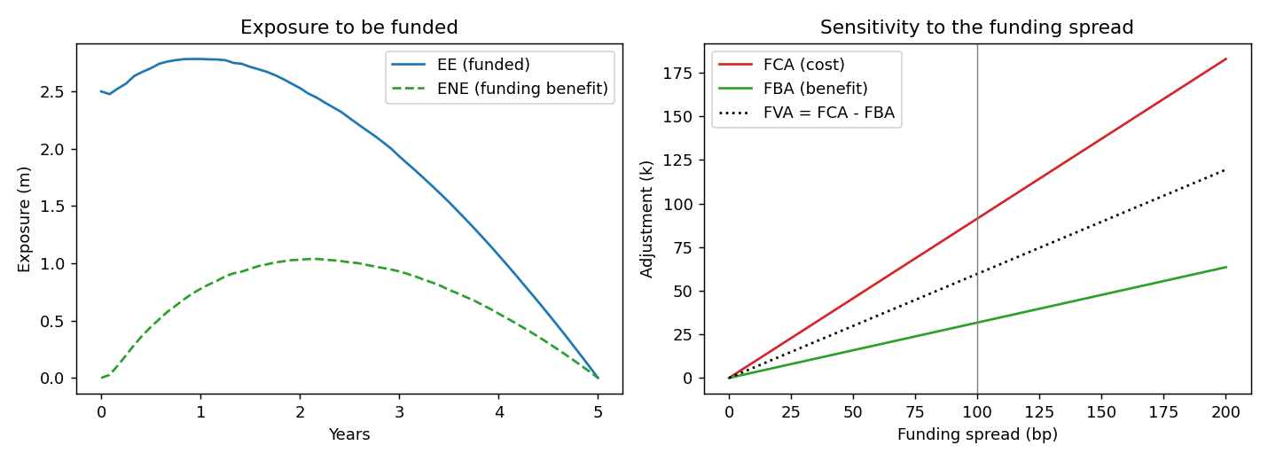
Exposure to be funded (left) and the sensitivity of FCA, FBA and FVA to the funding spread (right).#
Points to notice:
Because the swap is in the money, the expected exposure that has to be funded is well above the funding benefit, so the net FVA is a cost. The exposure at the start is not zero, as the trade has value on day one.
FVA is linear in the funding spread. Doubling the spread doubles each adjustment, so FVA is sensitive to the funding curve used, which is a matter of judgement.
If the swap were at par, the exposure would be symmetric. FCA and FBA would then nearly cancel and the net FVA would be close to zero. This is the effect behind the debate below, where netting the funding benefit against the cost is the main point of disagreement.
The FVA debate#
FVA is the most contested of the adjustments. The argument is about whether a bank’s own funding spread should be in the price of a derivative at all.
For FVA: a bank really does pay its funding spread to finance the uncollateralised exposure, so ignoring it overstates the profit on the trade.
Against FVA: when the bank owes money on the derivative, the same funding spread is a benefit, and that benefit is already captured by DVA. Counting both the funding cost and the DVA benefit double counts. In the classical corporate finance view, the funding cost of an asset should not depend on who the owner is.
In practice, many banks split FVA into a funding cost on positive exposure (FCA) and a funding benefit on negative exposure (FBA), and some net the benefit against DVA to avoid the overlap. The treatment differs between firms, so FVA is an area of valuation judgement that needs to be documented, reserved and reviewed.
FVA is one part of the wider XVA picture. It sits alongside CVA, DVA and KVA, each representing a different economic friction or adjustment that can affect the fair value of a derivative or portfolio. Taken together, these adjustments help bridge the gap between theoretical pricing and the actual economics of running a derivatives book.