CVA: Credit Valuation Adjustment#
Counterparty Credit Valuation Adjustment, or CVA, is the adjustment to the value of a derivative portfolio to reflect the risk that a counterparty may default and fail to pay amounts owed to the firm. In other words, CVA recognises that the expected future exposure to a counterparty is not always fully recoverable.
The starting point is the risk-free valuation of the trade. That value assumes no default risk. CVA then reduces the value of exposures that are positive to the firm when there is a possibility that the counterparty may default. If the trade is a receivable to the firm, the expected loss from counterparty default is a reduction in the mark. If the position is a payable, the logic is different and the exposure is typically viewed from the other side of the trade.
At a high level, CVA captures the expected loss due to counterparty default over the life of the transaction. The relevant drivers are:
the size of the exposure over time
the probability of default of the counterparty
the loss given default
the expected recovery rate
the distribution of exposure over the trade’s life
A common simplified intuition is:
where the expected exposure, default probability, recovery rate and discounting all vary over time. In practice, banks compute CVA using simulation-based or exposure profile methods that capture how the exposure changes as the trade evolves and as the market moves.
Why it matters#
CVA matters because it helps translate counterparty default risk into a cost that can be monitored, hedged and reported. It is a key ingredient in the fair value of OTC derivatives, especially for large portfolios where the counterparty concentration and exposure profile can change materially over time.
It also drives hedging decisions. Banks often hedge CVA risk using credit default swaps, index instruments or portfolio-level hedges, and the hedging strategy depends on how the exposure is distributed across counterparties, maturities and market factors.
CVA is usually discussed alongside DVA, FVA and KVA because the same derivative portfolio can carry several different economic adjustments at once. Each represents a different source of value adjustment, and the overall XVA picture is obtained by understanding all of them together.
DVA and bilateral CVA#
Debit Valuation Adjustment, or DVA, is the mirror image of CVA. CVA is the loss from the counterparty defaulting on what it owes us, and DVA is the gain from us defaulting on what we owe the counterparty. It uses the negative exposure profile (ENE) and the firm’s own default probability:
The two are combined into the bilateral CVA, which is the adjustment applied to the value of the portfolio:
so the value adjustment to the portfolio is \(-\text{CVA} + \text{DVA}\). Because the calculation is symmetric, a separate model is not needed, but the following points are not symmetric and need to be understood:
The sign of the P&L: if the firm’s own credit spread widens, its DVA increases and it books a gain. This is counterintuitive and is often questioned by management and auditors.
Hedging: CVA can be hedged by buying protection on the counterparty, but a firm cannot buy protection on its own default. DVA is therefore normally unhedged, or hedged only indirectly with proxies such as a basket of similar names, which carries basis risk.
Regulatory capital: under Basel III, DVA gains are removed from regulatory capital, so DVA is not available to absorb losses and provides no capital benefit.
Accounting: under IFRS 9, own-credit movements on liabilities designated at fair value go to other comprehensive income. Some firms therefore disclose or manage DVA separately from the rest of the P&L.
Overlap with FVA: the funding benefit that comes from a firm’s own credit spread is closely related to DVA, and counting both risks double counting. This is the basis of the debate described in FVA: Funding Valuation Adjustment.
A worked example#
The script below prices the CVA and DVA of a 5-year payer interest rate swap. It follows the steps in XVA: An Introduction to Valuation Adjustments:
Simulate the interest rate and revalue the swap at each month-end on 20,000 paths.
Aggregate the values into the exposure profiles: EE, ENE and the 95% PFE.
Convert the credit spreads into default probabilities for each month, using a constant hazard rate \(\lambda = s / (1 - R)\).
Sum \((1 - R) \times \text{EE} \times \text{PD} \times \text{DF}\) for CVA, and the same with ENE and the firm’s own credit for DVA.
The model is deliberately simple: a Gaussian rate, a swap valued as notional times remaining life times the rate move, a flat discount curve and no collateral. It shows the mechanics, not a production model.
"""Illustrative CVA and DVA for a 5-year payer interest rate swap."""
from pathlib import Path

import matplotlib
import numpy as np

matplotlib.use("Agg")
import matplotlib.pyplot as plt

rng = np.random.default_rng(42)

# Trade and market assumptions
notional = 100e6
maturity = 5.0
steps_per_year = 12
n_paths = 20_000
rate0 = 0.03        # flat rate; the fixed rate equals it, so the swap starts at par
rate_vol = 0.01     # normal (absolute) volatility of the rate, per sqrt(year)
disc_rate = 0.03    # flat discount rate

# Credit assumptions: spread / (1 - recovery) gives a constant hazard rate
cpty_spread, cpty_recovery = 0.0150, 0.40
own_spread, own_recovery = 0.0100, 0.40

# 1. Simulate the rate and value the swap at each future date.
#    Value ~ notional x remaining annuity x (rate - fixed rate).
dt = 1.0 / steps_per_year
t = np.arange(0.0, maturity + dt / 2, dt)
shocks = rng.standard_normal((n_paths, len(t) - 1)) * np.sqrt(dt)
rate = rate0 + rate_vol * np.concatenate([np.zeros((n_paths, 1)), shocks.cumsum(axis=1)], axis=1)
value = notional * (maturity - t) * (rate - rate0)

# 2. Exposure profiles
ee = np.maximum(value, 0.0).mean(axis=0)     # expected exposure (to us)
ene = np.maximum(-value, 0.0).mean(axis=0)   # expected negative exposure (to them)
pfe = np.percentile(np.maximum(value, 0.0), 95, axis=0)


# 3. Default probability in each interval and the discount factors
def default_prob(spread, recovery):
    survival = np.exp(-spread / (1.0 - recovery) * t)
    return survival[:-1] - survival[1:]


df = np.exp(-disc_rate * t[1:])
mid = lambda x: 0.5 * (x[:-1] + x[1:])

# 4. CVA = (1 - R) x sum( EE x PD x DF ), DVA uses ENE and our own credit
cva_terms = (1 - cpty_recovery) * mid(ee) * default_prob(cpty_spread, cpty_recovery) * df
dva_terms = (1 - own_recovery) * mid(ene) * default_prob(own_spread, own_recovery) * df
cva, dva = cva_terms.sum(), dva_terms.sum()

print(f"CVA            : {cva:12,.0f}  ({cva / notional * 1e4:5.1f} bp of notional)")
print(f"DVA            : {dva:12,.0f}  ({dva / notional * 1e4:5.1f} bp of notional)")
print(f"Bilateral CVA  : {cva - dva:12,.0f}  (CVA - DVA)")
print(f"Peak EE        : {ee.max():12,.0f}  at year {t[ee.argmax()]:.2f}")

# 5. Plot
fig, (ax1, ax2) = plt.subplots(1, 2, figsize=(11, 4))
ax1.plot(t, pfe / 1e6, label="PFE (95%)", color="tab:red")
ax1.plot(t, ee / 1e6, label="EE", color="tab:blue")
ax1.plot(t, ene / 1e6, label="ENE", color="tab:green", linestyle="--")
ax1.set(title="Exposure profile of a 5y payer swap", xlabel="Years", ylabel="Exposure (m)")
ax1.legend()

ax2.plot(t[1:], np.cumsum(cva_terms) / 1e3, label="CVA", color="tab:blue")
ax2.plot(t[1:], np.cumsum(dva_terms) / 1e3, label="DVA", color="tab:green")
ax2.set(title="Cumulative adjustment", xlabel="Years", ylabel="Adjustment (k)")
ax2.legend()

fig.tight_layout()
out = Path(__file__).parent / "images" / "cva_example.png"
out.parent.mkdir(exist_ok=True)
fig.savefig(out, dpi=130)

# 6. Plot a sample of the simulated swap values, with EE and ENE as the average of the
#    positive and negative parts across all paths
fig, ax = plt.subplots(figsize=(8, 4.5))
ax.plot(t, value[:40].T / 1e6, color="grey", alpha=0.35, linewidth=0.8)
ax.plot(t, ee / 1e6, color="tab:blue", linewidth=2.2, label="EE (average of the positive part)")
ax.plot(t, -ene / 1e6, color="tab:green", linewidth=2.2, linestyle="--", label="-ENE (average of the negative part)")
ax.axhline(0.0, color="black", linewidth=0.8)
ax.set(title="Simulated swap values (40 of 20,000 paths)", xlabel="Years", ylabel="Swap value (m)")
ax.legend(loc="upper left")
fig.tight_layout()
fig.savefig(out.with_name("cva_paths.png"), dpi=130)
Running it gives:
CVA            :       78,894  (  7.9 bp of notional)
DVA            :       53,216  (  5.3 bp of notional)
Bilateral CVA  :       25,679  (CVA - DVA)
Peak EE        :    1,710,716  at year 1.67
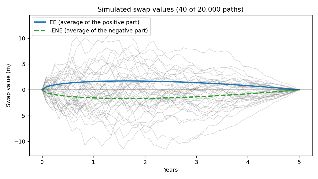
A sample of the simulated swap values. EE is the average of the positive part across all paths and ENE the average of the negative part.#
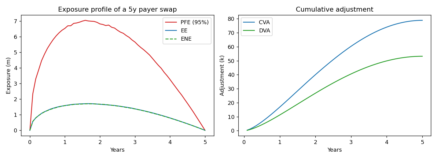
Exposure profile (left) and cumulative CVA and DVA (right).#
Points to notice:
The paths fan out from the starting value and then converge to zero at maturity, because the remaining cash flows run off. Averaging only the positive values gives EE, and averaging only the negative values gives ENE.
The exposure is hump shaped. It starts at zero because the swap is at par, grows as the rate diffuses, and falls back to zero as the remaining cash flows run off. The peak is at about year 1.7, not at the end of the trade.
The EE and ENE lines coincide because a par swap with a driftless rate is symmetric. Real portfolios are not, and the gap between the two lines is what drives the difference between CVA and DVA.
CVA is larger than DVA because the counterparty’s spread (150bp) is wider than ours (100bp). With equal spreads the two would be almost equal here, because the exposure is symmetric, and the bilateral CVA would be close to zero.
The PFE is several times the EE. This is why limits are set on PFE and valuation uses EE.