Hagan’s Approximation: From SABR to a Black Volatility#

The formula#

For a forward rate \(F\), strike \(K\) and expiry \(T\), the Black volatility is:

\[\sigma_B(K) = \frac{\alpha}{(FK)^{\frac{1-\beta}{2}} \left[ 1 + \frac{(1-\beta)^2}{24} \ln^2\frac{F}{K} + \frac{(1-\beta)^4}{1920} \ln^4\frac{F}{K} \right]} \cdot \frac{z}{x(z)} \cdot \left[ 1 + \left( \frac{(1-\beta)^2}{24} \frac{\alpha^2}{(FK)^{1-\beta}} + \frac{\rho \beta \nu \alpha}{4 (FK)^{\frac{1-\beta}{2}}} + \frac{2 - 3\rho^2}{24} \nu^2 \right) T \right]\]

with

\[z = \frac{\nu}{\alpha} (FK)^{\frac{1-\beta}{2}} \ln\frac{F}{K}, \qquad x(z) = \ln \left( \frac{\sqrt{1 - 2\rho z + z^2} + z - \rho}{1 - \rho} \right)\]

The three factors have separate roles:

The first is the leading term, which gives the level of volatility and the skew that comes from \(\beta\).
The second, \(z / x(z)\), adds the effect of \(\rho\) and \(\nu\) on the smile. It is a function of how far the strike is from the money, in units of volvol.
The third is a time correction, which is small for short expiries and grows with \(T\). It is a first-order expansion in time, which is why the formula weakens at long expiries.

At the money#

When \(K = F\), both \(z\) and \(x(z)\) are zero, and \(z / x(z)\) tends to 1. The formula reduces to:

\[\sigma_{ATM} = \frac{\alpha}{F^{1-\beta}} \left[ 1 + \left( \frac{(1-\beta)^2}{24} \frac{\alpha^2}{F^{2-2\beta}} + \frac{\rho \beta \nu \alpha}{4 F^{1-\beta}} + \frac{2 - 3\rho^2}{24} \nu^2 \right) T \right]\]

To a first approximation the at-the-money volatility is \(\alpha / F^{1-\beta}\). This is why \(\alpha\) can be solved from the at-the-money volatility during calibration. The code has to handle the \(z \to 0\) limit separately, because the ratio is \(0/0\).

From volatility to a price#

The steps to price a swaption at strike \(K\) are:

From the curve, compute the forward swap rate \(F\) and the annuity \(A\). See Interest Rate Curve Build.
Evaluate \(\sigma_B(K)\) using the formula and the calibrated parameters.
Put \(\sigma_B(K)\) in the Black-76 formula to get the price.

The model implementation is the function below. It is part of the script in SABR: Modelling the Volatility Smile, and the \(z \to 0\) case is handled with a safe division.

def sabr_black_vol(forward, strike, expiry, alpha, beta, rho, nu, shift=0.0):
    """Hagan et al. (2002) lognormal implied vol. A positive `shift` handles low or negative rates."""
    f, k = forward + shift, np.asarray(strike, dtype=float) + shift
    log_fk = np.log(f / k)
    fk_mid = (f * k) ** ((1.0 - beta) / 2.0)
    z = nu / alpha * fk_mid * log_fk
    sqrt_term = np.sqrt(1.0 - 2.0 * rho * z + z**2)
    x_z = np.log((sqrt_term + z - rho) / (1.0 - rho))
    # z / x(z) tends to 1 at the money, where both are zero.
    z_over_x = np.where(np.abs(z) < 1e-7, 1.0, z / np.where(np.abs(z) < 1e-7, 1.0, x_z))
    denominator = fk_mid * (1.0 + (1.0 - beta) ** 2 / 24.0 * log_fk**2 + (1.0 - beta) ** 4 / 1920.0 * log_fk**4)
    correction = 1.0 + (
        (1.0 - beta) ** 2 / 24.0 * alpha**2 / fk_mid**2
        + rho * beta * nu * alpha / (4.0 * fk_mid)
        + (2.0 - 3.0 * rho**2) / 24.0 * nu**2
    ) * expiry
    return alpha / denominator * z_over_x * correction

Normal volatility#

Hagan et al. also give an approximation for the normal volatility, which fits markets that quote in basis points. An alternative is to compute the Black price from the formula above, and then to find the normal volatility that returns the same price, which is what the scripts in this series do. For \(\beta = 0\) the model is already normal at the leading order.

Shifted SABR#

For rates that are close to zero or negative, replace \(F\) and \(K\) by \(F + s\) and \(K + s\), for a shift \(s\) of, for example, 1% to 3%. The function above has a shift argument that does this. The shift is a parameter of the methodology, and it must be the same in the calibration and in the pricing. A worked example, with a negative forward rate and a comparison of different shifts, is in SABR: Modelling the Volatility Smile.

Where the approximation fails#

The formula is an expansion, not the exact solution of the model. Problems appear in three situations:

Low strikes and long expiries. The implied density, which is the second derivative of the call price with respect to the strike, can become negative. This gives a price with an arbitrage, and a price that cannot be hedged.
Large volvol. The time correction grows, and the approximation moves away from the true model.
Very low rates. With a small \(F\), the formula is sensitive to the choice of \(\beta\) and the shift.

The script tests this by computing the density from the fitted parameters. For the 5-year expiry it is positive across strikes from 0.2% to 10%, and the lowest value is 0.887. Keeping the same parameters but using expiries of 20 and 30 years, the density becomes negative at low strikes:

Lowest density on 0.2% to 10% strikes: 0.887
Expiry    5Y: lowest density 0.887
Expiry   20Y: lowest density -71.446
Expiry   30Y: lowest density -66.633

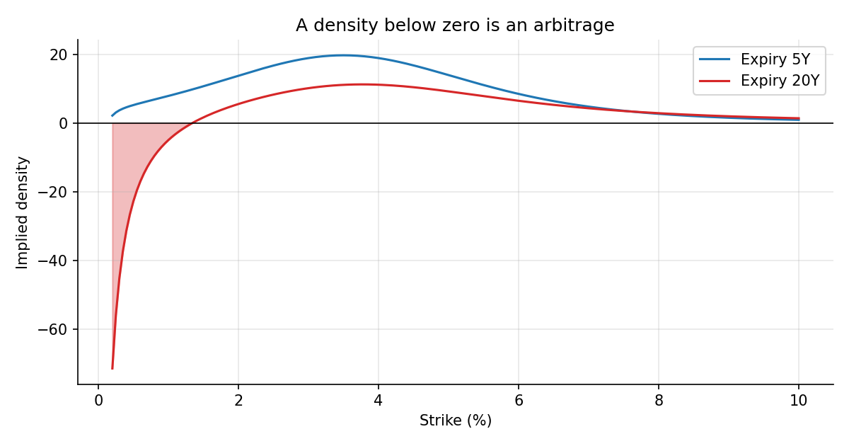
Implied density from the fitted SABR parameters for 5 and 20 year expiries, negative at low strikes for 20 years — The implied density at two expiries. The shaded area, where the density is negative, is an arbitrage.#

The longer-expiry lines are an illustration, since a real calibration would give different parameters for a 20 year expiry. They show the pattern that appears in practice for long-dated options at low strikes.

Fixes used in practice#

Restrict the range of strikes over which the formula is used, and extrapolate beyond it with a model that is arbitrage-free, such as a lognormal tail.
Arbitrage-free SABR, which replaces the approximation with a numerical solution of the model, such as a finite-difference solution of the density, with an absorbing boundary at zero.
Higher-order or improved expansions, such as the corrections that have been published since 2002.
Check and reject: a calibration whose implied density is negative anywhere in the range that is needed is flagged, and the parameters are refitted with a constraint.

A valuation control view#

Independent implementation: the approximation is reimplemented by the validation team, and the volatilities are compared with the front office to a tight tolerance. The ATM branch and the \(z \to 0\) limit are common sources of bugs.
Range of validity: the expiries, tenors and strikes for which the approximation is accepted are written down. Positions outside it are a model limitation, and they attract a reserve. See Prudent Valuation.
Density and convexity tests: run on every calibration, as in the script, with an exception if they fail.
Version control: the formula, the shift and the choice of \(\beta\) are part of the approved model. A change is a model change. See Governance: Model Risk, Accountability and Data.
Reporting: prices that depend on the smile far from the money are Level 3 inputs if the quotes are not observable. See Fair-value hierarchy: Levels 1, 2 & 3.