Curve Build, Part 2: Jacobians, Global Solvers and Multi-Curve#

Sequential bootstrap and global solve#

The bootstrap solves for one unknown at a time and never revisits a pillar. A global solver treats all the discount factors as one vector of unknowns \(x\) and solves for them together:

\[r_i(x) = \text{par rate}_i(x) - q_i = 0, \qquad i = 1, \dots, m\]

where \(q_i\) is the quote for instrument \(i\) and \(m\) is the number of instruments. The unknowns are normally the log discount factors, which keeps them positive. A Newton or Levenberg-Marquardt iteration then drives the residuals to zero.

Bootstrap compared with a global solve#
Aspect	Sequential bootstrap	Global solve
Unknowns	One at a time, shortest first.	All at once.
Instruments and knots	One instrument per knot, with an exact fit.	Any number of instruments, which can be more than the knots.
When quotes disagree	Cannot say. It reprices each in turn, and a bad quote spreads along the curve.	Gives a best fit in the least-squares sense, and the residuals show which quotes are out of line.
Interpolation	Local rules only, such as log-linear or monotone convex.	Any rule, including smooth splines that depend on all the knots.
Speed	Fast and simple.	Slower, and needs a good starting point, but also gives the Jacobian as a by-product.
Typical use	Prototype, or a liquid curve with one clean instrument per pillar.	Production curve sets, especially with several curves that depend on each other.

When the number of instruments equals the number of knots, the two methods give the same curve. When there are more instruments than knots, the problem is over-determined, and the solver minimises a weighted sum of squares:

\[\min_x \sum_i w_i \, r_i(x)^2 \; + \; \lambda \, R(x)\]

The weights \(w_i\) reflect the bid-offer spread or the reliability of each quote, so a liquid quote counts for more than a wide one. The optional term \(\lambda R(x)\) is a penalty for roughness, such as the integral of the squared change in the forward rate, and it trades fit for smoothness. This is a form of regularisation, and the amount \(\lambda\) is a methodology choice that should be documented.

The first two parts of the example show it. In part 1 the global solve with nine quotes and nine knots matches the bootstrap to \(10^{-12}\). In part 2 two extra quotes are added, at 4 and 6 years, that are slightly out of line with the others, and the curve is fitted to eleven quotes with the same nine knots:

1. Global solve vs bootstrap: largest DF difference 4.5e-13

2. Eleven quotes, nine knots (4Y and 6Y quoted 1.5bp high and 1.0bp low):
     1Y  residual  -0.00 bp
     2Y  residual  -0.00 bp
     3Y  residual  +0.42 bp
     4Y  residual  -1.12 bp
     5Y  residual  +0.35 bp
     6Y  residual  +0.85 bp
     7Y  residual  -0.50 bp
    10Y  residual  +0.00 bp
    15Y  residual  +0.00 bp
    20Y  residual  +0.00 bp
    30Y  residual  +0.00 bp

The curve no longer reprices the inputs exactly. The misfit of the two extra quotes is shared with their neighbours, and the residuals tell the curve owner which quotes to examine. A fit that leaves a residual is not an error. The question for control is whether the residuals are within the quote’s bid-offer spread.

The Jacobian#

The Jacobian is the matrix of derivatives of the repriced instruments with respect to the unknowns:

\[J_{ij} = \frac{\partial r_i}{\partial x_j}\]

It is used inside the solver, where the Newton step is \(x \leftarrow x - J^{-1} r\). It is also the key to curve risk.

Risk by input quote#

A trader wants to know how the value of a trade changes when each input quote moves, for example by one basis point. That is a bucketed, or key-rate, risk, and it is also what a hedge is built from, because each input is an instrument that can be traded. The curve is defined implicitly by \(r(x, q) = 0\), so the implicit function theorem gives the sensitivity of the curve to the quotes:

\[\frac{\partial x}{\partial q} = J^{-1}\]

Because the residual is the repriced rate less the quote, its derivative with respect to the quote is the identity. The risk of a trade with value \(V(x)\) then follows from the chain rule:

\[\frac{\partial V}{\partial q} = \frac{\partial V}{\partial x} \, J^{-1}\]

This gives the risk to every input from one matrix inverse, not one curve rebuild per input. With hundreds of inputs across a curve set, it is much faster, and it is exact, not a finite difference.

Example#

The script values a 6-year payer swap, struck at the 6-year par rate, on the curve from part 1. A 6-year swap is not one of the inputs, so its risk falls on the quotes on either side. The risk from the Jacobian is compared with bumping each quote by 1 basis point and rebuilding the curve:

3. Risk of a 6Y payer swap struck at par, per +1bp in each input (PV 0):
    Input    Jacobian     Rebuild
       1Y         0.2         0.2
       2Y         0.4         0.4
       3Y         1.0         1.0
       5Y    22,019.1    22,019.0
       7Y    30,925.5    30,926.7
      10Y         0.0        -0.0
      15Y         0.0        -0.0
      20Y         0.0        -0.0
      30Y         0.0        -0.0
    Total    52,946.3    52,947.3

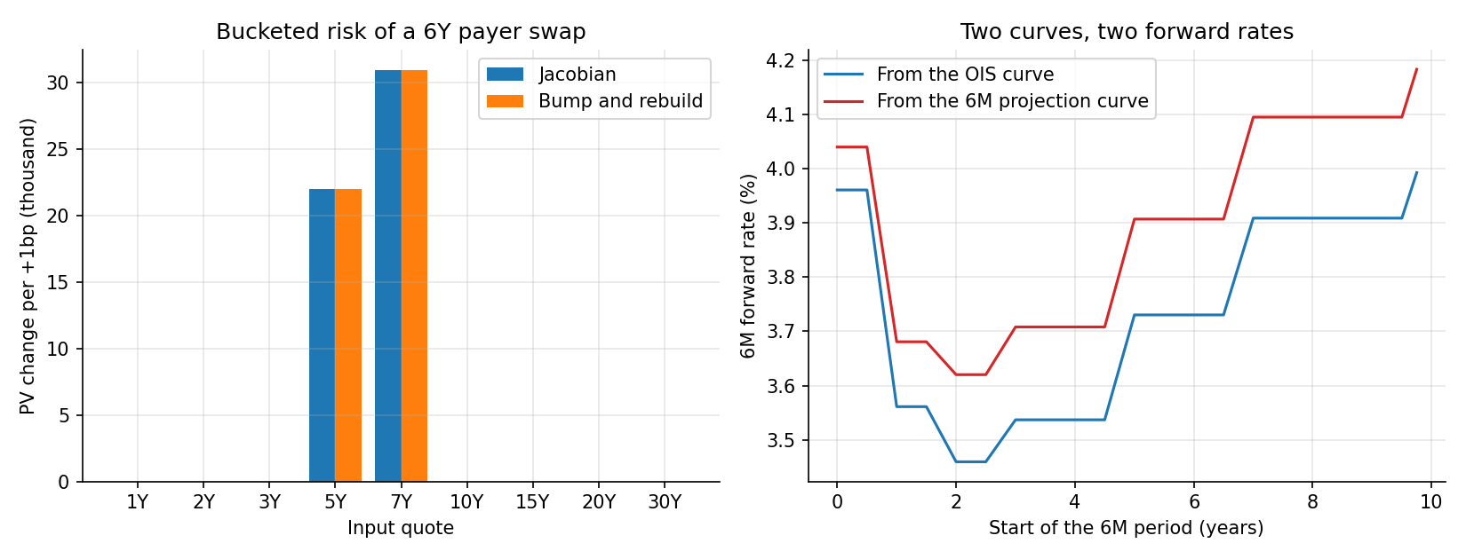
Bucketed risk from the Jacobian and from bumping, and forward rates from the OIS curve and the 6M projection curve — Left: the two ways of calculating bucketed risk agree. Right: forward rates of the 6M index from the two curves in the example below.#

Reading the output:

The risk sits on the 5-year and 7-year inputs, with 22,019 on the 5-year and 30,926 on the 7-year, because the 6-year discount factor is interpolated from the pillars either side. A trader would hedge with 5-year and 7-year swaps in those amounts.
The Jacobian and the rebuild agree. They differ by about one part in 50,000, because the Jacobian is the exact derivative and the bump is a finite 1 basis point change, which includes a small amount of convexity.
The short pillars have a small risk, because the 5-year discount factor depends on the earlier ones through the bootstrap.

The Jacobian is also used for scenario analysis, for hedging (solve for the amounts of the input instruments that offset the risk), and in XVA, where the sensitivities to the curve inputs of a whole portfolio are needed. Automatic differentiation computes the same quantities faster in large systems.

Interpolation and the stability of forwards#

The interpolation rule has a large effect on risk and on forward rates. With log-linear discount factors, the forward rate is flat between pillars and jumps at each pillar, as in the figure above. A bump to one quote moves the forward rates either side of the pillar by different, and sometimes opposite, amounts. The example shows it for the 6M index curve below: bumping the 5-year quote by 1 basis point moves the 6M forward starting at 5 years by -2.8 basis points. That kind of amplification and sign change in the forwards is known as a sawtooth. It makes the hedges of forward-starting trades unstable.

Smoother interpolation helps. Monotone convex and similar schemes (see the paper by Hagan and West) aim to keep forward rates positive and local while making them continuous. The trade-off is that a smooth rule can spread the risk of one quote over more pillars and, if poorly built, can oscillate. The choice has to be part of the documented methodology, and the same rule has to be used in every system that values trades off the curve.

Multi-curve#

Part 1 mentioned that one curve no longer serves for both discounting and projection. The modern set-up is:

a discount curve that follows the rate paid on collateral, which is an overnight rate such as SOFR, SONIA or the euro short-term rate
a projection curve for each index tenor that is still used, such as a 6-month index, which estimates the floating payments of swaps on that index

The projection curves are built on top of the discount curve. For a 6M-index swap with annual fixed payments, the pillar equation is

\[s \sum_{i} D(T_i) = \sum_{j} \left( \frac{P(t_{j-1})}{P(t_j)} - 1 \right) D(t_j)\]

where \(D\) is the discount curve, \(P\) is the projection curve and \(t_j\) are the half-yearly floating dates. The left side is the fixed leg. On the right, the term in brackets is the accrual times the forward rate of the index for the period, which is discounted with \(D\). The projection curve is solved for each pillar in turn, as in the bootstrap, but with the discount curve already known.

The difference between a forward rate from the projection curve and one from the discount curve is the tenor basis: the market price of the difference in credit and liquidity between lending for six months and rolling overnight. In the example, the 6M swap rates are 8 to 17 basis points above the overnight swap rates, and the 6M forward starting at 5 years is 3.907% from the projection curve against 3.730% from the discount curve.

Dependencies between curves#

The curves cannot be solved separately if they depend on each other. The example tests both directions:

4. 6M index swap rates and the forward rate of the 6M index, starting 5Y out:
   OIS-discounted 6M forward 3.7303%, projection curve 3.9070%
   Bump the 5Y OIS quote by 1bp, 6M quotes held: the 6M forward at 5Y moves +0.03 bp
   Bump the 5Y 6M quote by 1bp, OIS held: the 6M forward at 5Y moves -2.81 bp (the OIS curve is solved first, so it cannot move)

The projection curve depends on the discount curve, because the floating leg is discounted with it, so a move in the overnight quote has a small effect on the 6M curve (0.03 basis point here). The discount curve does not depend on the projection curve. The Jacobian of the whole curve set is therefore block triangular, with the discount curve in the first block.

In production the curves often depend on each other in both directions, for example when a basis swap pays one index and is collateralised in another, or when a cross-currency swap links two curve sets. Then the whole set is solved together with a global solver, and the Jacobian across the set gives the risk of each trade to every input in every curve.

Other practical points#

Futures and FRAs: futures prices need a convexity adjustment to turn them into forward rates, and the adjustment depends on a volatility assumption.
Turn-of-year and month-end effects: the overnight rate jumps over the year end and quarter ends. A smooth interpolation cannot reproduce that, and so the short end often has explicit jump or “turn” adjustments.
Cross-currency and collateral: the discount curve for a trade depends on the currency of the collateral, and a cross-currency basis curve links markets. See ColVA: Collateral Valuation Adjustment.
Extrapolation: beyond the last liquid quote the curve is an assumption, such as a flat last forward or a convergence to an ultimate forward rate, and it needs its own governance. Long-dated risk can be large.
Quotes versus prices: a curve can be built from par rates, as here, or from instrument prices, which handles stub periods, off-market swaps and different payment dates properly.
Snapshots and timing: all the quotes must come from the same time. A stale quote in a global fit spreads its error into the neighbours.

A valuation control view#

Rebuild independently. Rebuild the curve with a different solver or tool, and compare the discount factors and the par rates. The first example above is a small version of this test, as it compares a global solve with a bootstrap.
Review the residuals. For a global fit, the residual by instrument is reviewed against a tolerance based on the bid-offer. A growing residual on one quote is an input problem to investigate.
Reconcile the risk. Compare the Jacobian risk of a test trade with the risk from bumping, as in the output above, and with the risk system. A break points to a different interpolation, a different set of inputs, or a bug.
Check the forwards. Look for sawtooth patterns and negative forwards, and test the effect of a one basis point bump on the forwards around each pillar.
Document the choices. The instruments in each pillar, the weights, the interpolation, any smoothing, the turn adjustments and the extrapolation are all part of the methodology. See Governance: Model Risk, Accountability and Data.
Consistency across systems. A curve built one way for pricing and another way for risk will produce risk that does not match the P&L. The rule is one methodology, applied everywhere.
Link to reserves and levels. Quotes for long maturities and for illiquid basis curves may not be observable, which affects the level and the valuation reserves. See Fair-value hierarchy: Levels 1, 2 & 3.

The script#

"""Beyond the basic bootstrap: a global solver, curve risk from the Jacobian, and a second curve."""
import numpy as np
from scipy.optimize import brentq, least_squares

from curve_example import PAR_RATES, PILLARS, Curve, bootstrap, forward_swap

N = 100e6


def curve_from(x, knots=PILLARS):
    """A curve whose unknowns are the log discount factors at the knots."""
    return Curve(np.array(knots, dtype=float), np.exp(x))


def par_rates(curve, maturities):
    return np.array([forward_swap(curve, 0, int(m))[0] for m in maturities])


def solve_global(maturities, quotes, knots=PILLARS):
    """Fit every quote at once. With more quotes than knots this is a least-squares fit."""
    residuals = lambda x: par_rates(curve_from(x, knots), maturities) - quotes
    fit = least_squares(residuals, -0.035 * np.array(knots, dtype=float), method="lm", xtol=1e-14, ftol=1e-14)
    return fit.x, fit.fun


def jacobian(function, x, step=1e-6):
    """Central-difference Jacobian of a vector function."""
    columns = []
    for i in range(len(x)):
        up, down = x.copy(), x.copy()
        up[i] += step
        down[i] -= step
        columns.append((function(up) - function(down)) / (2 * step))
    return np.array(columns).T


def payer_pv(curve, maturity, strike):
    """PV of paying fixed against an overnight floating leg, per unit notional."""
    return (1.0 - curve.df(maturity)) - strike * curve.df(np.arange(1, maturity + 1)).sum()


def projection_curve(discount, maturities, quotes):
    """Bootstrap a 6M-index curve on top of an OIS discount curve (annual fixed, semi-annual floating)."""
    times, dfs = [], []
    for T, s in zip(maturities, quotes):

        def error(p_T):
            proj = Curve(times + [T], dfs + [p_T])
            half_years = np.arange(0.5, T + 0.25, 0.5)
            previous = np.concatenate([[0.0], half_years[:-1]])
            floating = ((proj.df(previous) / proj.df(half_years) - 1.0) * discount.df(half_years)).sum()
            fixed = s * discount.df(np.arange(1, T + 1)).sum()
            return fixed - floating

        dfs.append(brentq(error, 0.01, 1.0))
        times.append(T)
    return Curve(times, dfs)


def forward_6m(curve, start):
    return (curve.df(start) / curve.df(start + 0.5) - 1.0) / 0.5


if __name__ == "__main__":
    quotes = np.array(PAR_RATES)
    base = bootstrap()

    # 1. The global solver gives the bootstrap's answer when there are as many quotes as unknowns.
    x, residual = solve_global(PILLARS, quotes)
    largest = np.max(np.abs(np.exp(x) - base.df(np.array(PILLARS))))
    print(f"1. Global solve vs bootstrap: largest DF difference {largest:.1e}\n")

    # 2. More quotes than knots: the fit can no longer reprice everything.
    extra_maturities = [4, 6]
    implied = par_rates(base, extra_maturities)
    extra_quotes = implied + np.array([0.00015, -0.00010])
    all_maturities = list(PILLARS) + extra_maturities
    all_quotes = np.concatenate([quotes, extra_quotes])
    x_fit, residual = solve_global(all_maturities, all_quotes)
    order = np.argsort(all_maturities)
    print("2. Eleven quotes, nine knots (4Y and 6Y quoted 1.5bp high and 1.0bp low):")
    for i in order:
        print(f"   {all_maturities[i]:>3}Y  residual {residual[i] * 1e4:+6.2f} bp")

    # 3. Curve risk from the Jacobian, checked against a full rebuild for every quote.
    #    A 6Y swap is not one of the inputs, so its risk falls on the 5Y and 7Y quotes either side.
    quote_fn = lambda x_: par_rates(curve_from(x_), PILLARS)
    j_x = jacobian(quote_fn, x)                       # d(par rates)/d(log DFs)
    d_x_d_quote = np.linalg.inv(j_x)                  # d(log DFs)/d(quotes), by the implicit function theorem
    strike = forward_swap(base, 0, 6)[0]
    pv_fn = lambda x_: N * payer_pv(curve_from(x_), 6, strike)
    d_pv_d_x = jacobian(lambda x_: np.array([pv_fn(x_)]), x)[0]
    jacobian_risk = d_pv_d_x @ d_x_d_quote * 1e-4     # per +1bp in each quote

    bumped_risk = []
    for i in range(len(PILLARS)):
        bumped = quotes.copy()
        bumped[i] += 1e-4
        bumped_curve = bootstrap(PILLARS, bumped)
        bumped_risk.append(N * payer_pv(bumped_curve, 6, strike) - pv_fn(x))
    print(f"\n3. Risk of a 6Y payer swap struck at par, per +1bp in each input (PV {pv_fn(x):,.0f}):")
    print(f"   {'Input':>6} {'Jacobian':>11} {'Rebuild':>11}")
    for maturity, jac, bump in zip(PILLARS, jacobian_risk, bumped_risk):
        print(f"   {maturity:>5}Y {jac:11,.1f} {bump:11,.1f}")
    print(f"   {'Total':>6} {jacobian_risk.sum():11,.1f} {np.sum(bumped_risk):11,.1f}")

    # 4. A second curve for a 6M index, solved on top of the discount curve.
    spreads = np.array([8, 10, 12, 14, 15, 16, 17, 17, 17]) / 1e4
    six_month_quotes = quotes + spreads
    proj = projection_curve(base, PILLARS, six_month_quotes)
    print("\n4. 6M index swap rates and the forward rate of the 6M index, starting 5Y out:")
    print(f"   OIS-discounted 6M forward {forward_6m(base, 5.0):.4%}, projection curve {forward_6m(proj, 5.0):.4%}")

    bumped_ois = bootstrap(PILLARS, np.where(np.array(PILLARS) == 5, quotes + 1e-4, quotes))
    proj_after_ois_bump = projection_curve(bumped_ois, PILLARS, six_month_quotes)
    move = (forward_6m(proj_after_ois_bump, 5.0) - forward_6m(proj, 5.0)) * 1e4
    print(f"   Bump the 5Y OIS quote by 1bp, 6M quotes held: the 6M forward at 5Y moves {move:+.2f} bp")

    bumped_six = six_month_quotes + np.where(np.array(PILLARS) == 5, 1e-4, 0.0)
    proj_after_six_bump = projection_curve(base, PILLARS, bumped_six)
    move = (forward_6m(proj_after_six_bump, 5.0) - forward_6m(proj, 5.0)) * 1e4
    print(f"   Bump the 5Y 6M quote by 1bp, OIS held: the 6M forward at 5Y moves {move:+.2f} bp (the OIS curve is solved first, so it cannot move)")