Range Accruals, Digitals and the Wedge#
A range accrual pays a coupon only for the days on which a reference rate fixes inside a range. It is a popular structured note, because it pays a high coupon when the investor expects rates to stay quiet. It is also a product where the model used for the pricing and the way of handling the barrier both change the price and the risk, so it shows well what valuation control has to look at beyond the vanilla swaptions in Swaptions and the Black-76 Model.
The product#
A typical note pays a coupon on each date of
where \(C\) is the coupon rate, \(\tau\) is the accrual fraction, and a day is “in the range” if the reference rate \(R\) fixes between a lower level \(L\) and an upper level \(U\). The reference is often a 3 or 6 month rate, or a swap rate (a CMS rate), observed daily.
The investor buys the note and receives the coupons. The bank that sells it pays them, so the bank is short the in-range event: it loses when the rate is inside the range on many days. The note is often also callable by the bank, which adds a Bermudan option (see Bermudan Swaptions and Mean Reversion).
Decomposition into digitals#
Each fixing pays 1 if \(L \le R \le U\), which is the difference of two digital options, each paying 1 if the rate is above a level:
So a range accrual with 60 monthly fixings is a strip of 120 digitals. A digital is the limit of a call spread: a long call at \(K - \epsilon\) and a short call at \(K + \epsilon\), divided by \(2\epsilon\). As \(\epsilon \to 0\) the price is minus the slope of the call price with respect to the strike:
With a Black volatility that depends on the strike (a smile), the derivative has two parts:
The first term is the value with a flat volatility. The second is the skew correction: the vega of the call times the slope of the smile. For a smile that slopes down, which is typical, the correction is positive. This is why the smile model from SABR: Modelling the Volatility Smile is part of the price of a digital.
The smile matters#
The script prices a five-year note with a 5% coupon and monthly fixings of the 6-month rate, in the range 3.00% to 4.50%, for 100 million. The forward rates come from the curve in Interest Rate Curve Build, and the smile is a SABR smile with a 28% at-the-money volatility, \(\beta = 0.5\), \(\rho = -0.2\) and \(\nu = 0.5\). Those parameters are invented for the illustration.
Five-year range accrual, 5% coupon, 6M rate in [3.00%, 4.50%], monthly fixings

   Wedge    Mid value  Upper bound  Lower bound    Reserve
 digital   10,252,166
      5bp   10,251,249   10,517,549    9,979,449    266,300
     10bp   10,248,499   10,775,679    9,699,342    527,180
     25bp   10,229,281   11,507,631    8,814,613  1,278,350
     50bp   10,161,122   12,594,221    7,198,434  2,433,098

With a flat vol instead of the smile the digital value is 8,864,686, a difference of +1,387,480.

Delta of one fixing's digital at the lower barrier, as a % of its coupon notional, per +1bp in the forward:
  Time to fixing   Digital  10bp wedge  25bp wedge
         1 month     1.65%       1.64%       1.58%
          1 week     3.43%       3.32%       2.87%
           1 day     9.06%       7.44%       3.98%
The last line of the first block is the point on the smile. Pricing the same digitals with the single at-the-money volatility gives 8.86 million, against 10.25 million with the smile, a difference of 1.39 million, or 14% of the value. The note is worth much more or much less depending on the skew, and the skew at strikes of 3% and 4.5% on a five-year horizon is usually not a liquid quote. The smile at those strikes is therefore a key input, and a likely source of Level 3 classification. See Fair-value hierarchy: Levels 1, 2 & 3.
Pin risk#
A digital pays 1 or 0 with nothing between, so its delta, the change in value for a small change in the rate, becomes extremely large when the rate is close to the barrier on the fixing date. This is pin risk: the rate is “pinned” near the barrier, and a small move changes the payoff from 0 to a whole coupon.
The last table shows it. One month before the fixing, a digital at the money has a delta of 1.65% of notional for a 1 basis point move. One day before, it is 9.06%. At the fixing it would be infinite. A trader hedging the digital with the underlying rate would have to buy and sell very large amounts each day for a payoff that is uncertain until the last minute. With a daily-fixing note there are many such barriers near the money at any time, and the hedging cost and risk are real.
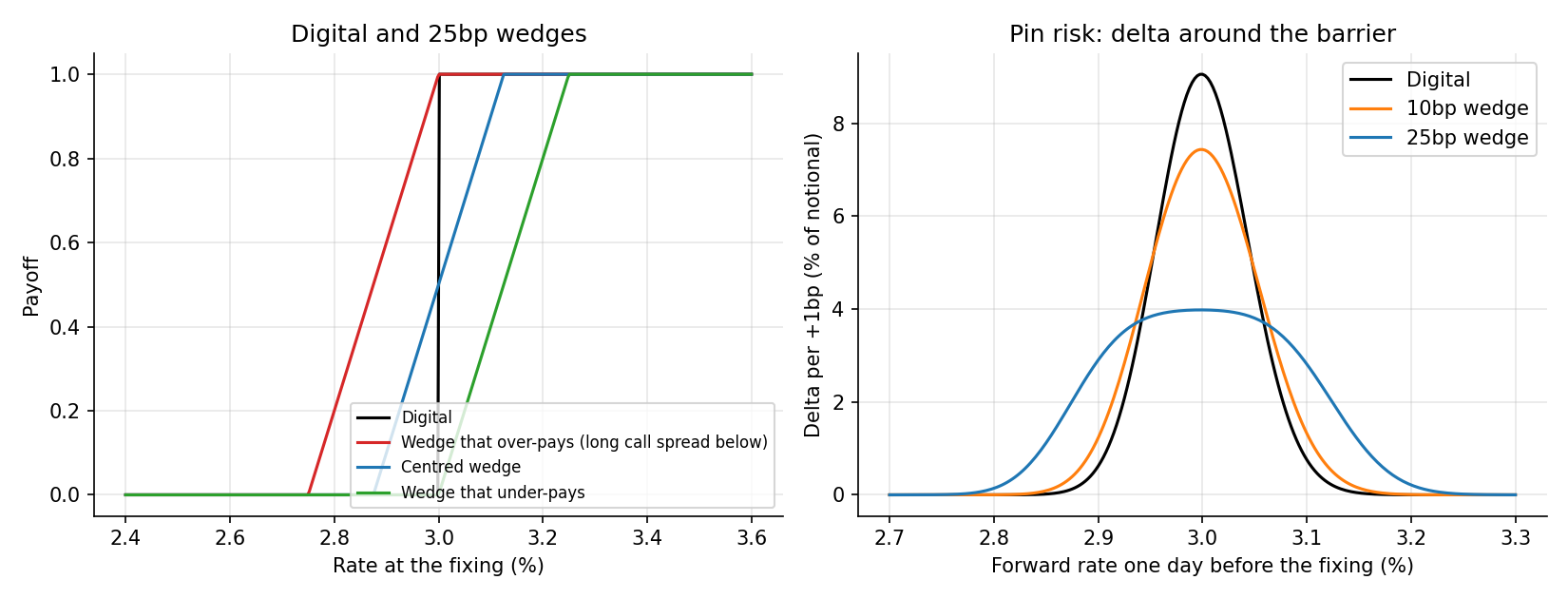
Left: the digital and three 25bp wedges. Right: the delta one day before the fixing. The digital’s delta is a sharp spike, and the wedge flattens it.#
The wedge#
The standard remedy is to replace each digital with a call spread, which is a digital with a sloped edge instead of a jump. The width of the slope, \(w\), is the wedge. The payoff is 0 below the lower strike, rises linearly across the wedge, and is 1 above the upper strike:
The slope inside the wedge is \(1/w\), so the delta is at most \(1/w\) per unit of rate, however close the fixing is. In the table, a 25 basis point wedge limits the delta to about 4% of the notional per basis point, against 9% for the digital with one day to go. The trader can hedge with real option strikes, a long call and a short call, which are quoted and tradeable.
Where to put the wedge#
There are three ways to place a wedge of width \(w\) around the barrier \(K\):
Centred: strikes at \(K \pm w/2\). This is closest to the digital, and gives the mid price.
Over-paying: strikes at \(K - w\) and \(K\). The payoff is always at least that of the digital, so it is conservative for the party that is short the digital, and it gives an upper bound.
Under-paying: strikes at \(K\) and \(K + w\). The payoff is never more than the digital’s, and it gives a lower bound.
For the note, the bank is short the range, so it pays when the rate is inside. The range is a difference of two digitals, so the over-paying (conservative) bound for the bank uses an over-paying wedge on the lower barrier, which adds to the payoff, and an under-paying wedge on the upper barrier, which subtracts less. The “Upper bound” column in the table is that bound, and “Lower bound” is the opposite.
Reading the table#
The mid value hardly moves with the wedge. A 25 basis point centred wedge changes the value from 10.25 million to 10.23 million. The smoothing barely changes the central price.
The bounds widen quickly. The spread between the upper and lower bounds grows in proportion to the wedge, from about 0.54 million at 5 basis points to about 5.4 million at 50. That range is the price of not knowing the exact behaviour at the barrier.
The reserve is the upper bound less the mid value. A bank that wants to be conservative on the liability takes a reserve of that size, 0.53 million at 10 basis points and 1.28 million at 25 basis points. It can be seen as the cost of the pin risk that remains when the hedge is a call spread, and not a digital.
The delta is capped. The wedge turns an unmanageable delta into a manageable one, at the price of a hedge that no longer matches the payoff exactly inside the wedge.
Choosing the width#
Liquidity and cost of the hedge: a wedge that is too narrow gives a hedge that is too large and expensive to rebalance. A wide one leaves a large unhedged payoff.
Size of the position: the delta limit, per basis point, sets the smallest acceptable wedge for the notional.
Time to the fixing: some desks widen the wedge as the fixing approaches, so that the delta stays within limits.
Consistency: the wedge must be the same in the front office model, the risk system and the independent valuation, or the prices and Greeks will not reconcile.
Other points#
Payment lag and timing: the coupon is paid on a different date from the fixing. A proper model adjusts for that. The script discounts at the payment date and takes the probability under the fixing-date forward measure, which is an approximation.
CMS and spread range accruals: if the reference is a swap rate, there is a convexity adjustment, and if it is a spread between two rates, the correlation between them is a key input.
Callable range accruals: the bank’s right to call is a Bermudan option on the whole structure. It needs a multi-factor model that fits the smile, such as a market model, and so is a harder version of the problem in Bermudan Swaptions and Mean Reversion.
Hedging: the risks are to the rate, to volatility at each strike (vega by strike), and to the skew. A hedge uses swaps and a strip of caps, floors or swaptions.
A valuation control view#
Smile inputs: the volatilities at the barrier strikes, for the whole life of the note, are checked against independent data, and the extrapolation beyond the liquid strikes is reviewed. The skew correction above can be a tenth of the value.
Wedge methodology: the width and placement are part of the approved model. A change in the width is a model change, and the reserve is reported. See Governance: Model Risk, Accountability and Data.
Reserve: the difference between the conservative and mid value is a candidate model reserve for the bridge from the desk mark to fair value. See Financial Statements and Prudent Valuation.
Level: the value depends on an unobservable skew far from the money, so many range accruals are Level 3. Reasonable alternative inputs are tested, which gives the sensitivity disclosure. See Fair-value hierarchy: Levels 1, 2 & 3.
Day-one profit: a high margin on a note with unobservable inputs is deferred. See IFRS 9: Financial Instruments.
Independent replication: an independent calculation of the same strip of digitals, with a different wedge, shows how much of the price depends on that choice.
The script#
"""A range accrual note priced from digitals, with a call-spread wedge to smooth the pin risk."""
import numpy as np
from scipy.stats import norm

from curve_advanced_example import forward_6m
from curve_example import bootstrap
from sabr_example import sabr_black_vol

BETA, RHO, NU, ATM_VOL = 0.5, -0.20, 0.50, 0.28


def smile_vol(forward, strike, expiry, flat=False):
    """SABR vol with alpha set so the at-the-money Black vol is about 28%. `flat` removes the smile."""
    alpha = ATM_VOL * forward ** (1.0 - BETA)
    atm = float(sabr_black_vol(forward, forward, expiry, alpha, BETA, RHO, NU))
    if flat:
        return atm
    return float(sabr_black_vol(forward, strike, expiry, alpha, BETA, RHO, NU))


def call(forward, strike, expiry, flat=False):
    """Undiscounted Black call on the forward rate, with a strike-dependent vol."""
    sd = smile_vol(forward, strike, expiry, flat) * np.sqrt(expiry)
    d1 = (np.log(forward / strike) + 0.5 * sd**2) / sd
    return forward * norm.cdf(d1) - strike * norm.cdf(d1 - sd)


def prob_above(forward, strike, expiry, width=0.0, mode="centre", flat=False):
    """Probability (or its call-spread replacement) that the rate fixes above `strike`.

    width = 0 is the pure digital, the negative slope of the call price in strike, so the smile is included.
    A wedge replaces it with a call spread of that width:
      centre: strikes K -/+ width/2 (the mid price),
      over:   strikes K - width and K (pays at least the digital),
      under:  strikes K and K + width (pays at most the digital).
    """
    if width == 0.0:
        h = 1e-6
        return -(call(forward, strike + h, expiry, flat) - call(forward, strike - h, expiry, flat)) / (2 * h)
    lo, hi = {"centre": (strike - width / 2, strike + width / 2),
              "over": (strike - width, strike),
              "under": (strike, strike + width)}[mode]
    return (call(forward, lo, expiry, flat) - call(forward, hi, expiry, flat)) / (hi - lo)


def in_range(forward, lower, upper, expiry, width=0.0, side="mid", flat=False):
    """Probability that the rate fixes in [lower, upper]. side='high' gives an upper bound on the payoff."""
    if side == "mid":
        return prob_above(forward, lower, expiry, width, "centre", flat) - prob_above(forward, upper, expiry, width, "centre", flat)
    modes = ("over", "under") if side == "high" else ("under", "over")
    return prob_above(forward, lower, expiry, width, modes[0], flat) - prob_above(forward, upper, expiry, width, modes[1], flat)


def note_value(curve, lower, upper, coupon, width=0.0, side="mid", flat=False, years=5, fixings_per_year=12):
    """Value, per unit notional, of the coupons of a range accrual: coupon x share of fixings inside the range."""
    total = 0.0
    for k in range(years * fixings_per_year):
        t = k / fixings_per_year
        if t == 0.0:
            continue
        forward = forward_6m(curve, t)
        pay = t + 1.0 / fixings_per_year
        total += coupon / fixings_per_year * curve.df(pay) * in_range(forward, lower, upper, t, width, side, flat)
    return total


if __name__ == "__main__":
    curve = bootstrap()
    lower, upper, coupon = 0.030, 0.045, 0.05   # pays 5% p.a. for each fixing of the 6M rate between 3.0% and 4.5%
    notional = 100e6

    print("Five-year range accrual, 5% coupon, 6M rate in [3.00%, 4.50%], monthly fixings\n")
    print(f"{'Wedge':>8} {'Mid value':>12} {'Upper bound':>12} {'Lower bound':>12} {'Reserve':>10}")
    for width_bp in (0, 5, 10, 25, 50):
        w = width_bp / 1e4
        mid = note_value(curve, lower, upper, coupon, w, "mid") * notional
        high = note_value(curve, lower, upper, coupon, w, "high") * notional
        low = note_value(curve, lower, upper, coupon, w, "low") * notional
        label = "digital" if width_bp == 0 else f"{width_bp}bp"
        if width_bp == 0:
            print(f"{label:>8} {mid:12,.0f} {'':>12} {'':>12} {'':>10}")
        else:
            print(f"{label:>8} {mid:12,.0f} {high:12,.0f} {low:12,.0f} {high - mid:10,.0f}")

    flat = note_value(curve, lower, upper, coupon, 0.0, "mid", flat=True) * notional
    smile = note_value(curve, lower, upper, coupon, 0.0, "mid") * notional
    print(f"\nWith a flat vol instead of the smile the digital value is {flat:,.0f}, a difference of {smile - flat:+,.0f}.")

    # Pin risk: the delta of one monthly digital at the barrier as the fixing approaches.
    print("\nDelta of one fixing's digital at the lower barrier, as a % of its coupon notional, per +1bp in the forward:")
    print(f"{'Time to fixing':>16} {'Digital':>9} {'10bp wedge':>11} {'25bp wedge':>11}")
    for label, t in (("1 month", 1 / 12), ("1 week", 1 / 52), ("1 day", 1 / 365)):
        row = []
        for width in (0.0, 0.0010, 0.0025):
            up = prob_above(lower + 0.5e-4, lower, t, width)
            down = prob_above(lower - 0.5e-4, lower, t, width)
            row.append((up - down) * 100)
        print(f"{label:>16} {row[0]:8.2f}% {row[1]:10.2f}% {row[2]:10.2f}%")